QHack 2023: 4 week prep challenge, day 4, Givens rotations

Today, I’m heading again for a prepared exercise, the next exercise in the QHack 2022 Quantum Chemistry track. It requires slightly more preparation, than the previous two, but again very doable.

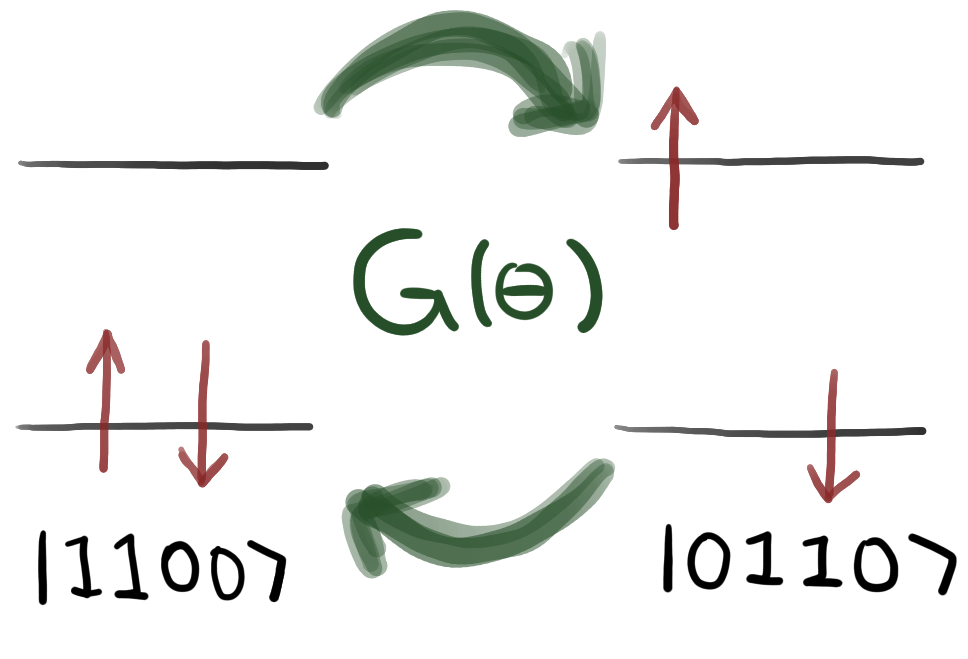
The challenge, invites to get more acquainted with Givens rotations, i.e. operations that allow to transform states, while preserving the hamming weight (the number of ones and zeros). They are the basic building blocks of quantum chemistry and “can be used to construct any kind of particle-conserving circuit”.

The goal is to find the correct rotation angles to transform a start state to a target state, with a quantum circuit with three Givens rotations,

\[|\Psi \rangle = CG^{(1)}(\theta_3; 0,1,3) G^{(2)}(\theta_2; 2,3,4,5) G^{(2)}(\theta_1; 0,1,2,3) |110000\rangle = \\ a |110000\rangle + b |001100 \rangle + c |000011 \rangle + d |100100\rangle \]

Getting to know Givens rotations

Givens rotations, describe transitions of electrons from a starting state to an excited state. In Pennylane, these rotations can be used via the classes qml.SingleExcitation and qml.DoubleExcitation. The linked tutorial is very recommendable.

A Givens rotation can be used to couple states that differ by a single excitation. Image taken from the Xanadu tutorial on Givens rotations.

Solving the exercise

To solve this exercise, I used the rotations’ transformation rules to reach an expression that associated trigonometric functions with the target factors. Further, I used the fact, that states are normalized at any time during the calculation. Key for me to solve it, was to apply only the first two rotations and used the normalization property of the state, from this I obtained the first angle. Then I went on to apply the remaining rotation and easily expressed the missing two angles.

import numpy as np


def givens_rotations(a, b, c, d):
    """Calculates the angles needed for a Givens rotation to out put the state with amplitudes a,b,c and d

    Args:
        - a,b,c,d (float): real numbers which represent the amplitude of the relevant basis states (see problem statement). Assume they are normalized.

    Returns:
        - (list(float)): a list of real numbers ranging in the intervals provided in the challenge statement, which represent the angles in the Givens rotations,
        in order, that must be applied.
    """

    theta1 = 2.*np.arccos(np.sqrt(1-b**2-c**2))
    theta2 = 2.*np.arcsin(c/np.sin(theta1/2.))
    theta3 = 2.*np.arccos(a/np.cos(theta1/2.))
    
    return [theta1, theta2, theta3]

Test

Defining the circuit…

import pennylane as qml

dev = qml.device('default.qubit', wires=6)

@qml.qnode(dev)
def circuit(x, y, z):
    qml.BasisState(np.array([1, 1, 0, 0, 0, 0]), wires=[i for i in range(6)])
    qml.DoubleExcitation(x, wires=[0, 1, 2, 3])
    qml.DoubleExcitation(y, wires=[2, 3, 4, 5])
    # single excitation controlled on qubit 0
    qml.ctrl(qml.SingleExcitation, control=0)(z, wires=[1, 3])
    return qml.state()

and executing the circuit …

[x, y, z] = givens_rotations(0.8062,-0.5,-0.1,-0.3)
circuit(x,y,z)

yields the correct amplitudes, success!

Transformation rules

Double excitation

\[ G^{(2)} (\theta; 1,2,3,4) |0011\rangle = \cos{\frac{\theta}{2}} |0011\rangle + \sin{\frac{\theta}{2}} |1100\rangle \\ G^{(2)} (\theta; 1,2,3,4) |1100\rangle = \cos{\frac{\theta}{2}} |1100\rangle – \sin{\frac{\theta}{2}} |0011\rangle \\ \]

Controlled single excitation

\[ CG(\theta; 0,1,2)|101\rangle = \cos{\frac{\theta}{2}}|101\rangle + \sin{\frac{\theta}{2}}|110\rangle \\ CG(\theta; 0,1,2)|110\rangle = \cos{\frac{\theta}{2}}|110\rangle – \sin{\frac{\theta}{2}}|101\rangle \]

QHack 2023: 4 week prep challenge, day 3, Clustering measurements

I felt I had some unfinished business on yesterday’s exercise, so I drafted an improved optimization routine. I formulated an ad hoc hypothesis, that shows in a small-scale test some improvements over the original optimization scheme.

An important observation: order matters

Two measurements can be combined, if they fulfill certain criteria, cf. yesterdays post. However, if you combine measurements locally using a greedy procedure, you might end up with sub-optimal combinations, and requiring more measurements eventually.

If you number your measurements 1 .. N as nodes in a graph and edges between nodes, if you can perform them in parallel, you may end up with a graph like the following.

Maximum clique graph, taken from here.

Given this graph, you immediately see a large clique (a fully connected subgraph, nodes 1, 2, 4, 5, 7, 11), that you would instinctively replace with a single measurement right away. You’d continue with the remaining cliques (3, 9, 10 and 8, 6), three measurements in total. The order of replacement is key, if by chance you’d join up the nodes 5, 6, 10 first, you’d end up with 4 measurements in total.

Create the graph

Using the networkx package, I created the aforementioned undirected graph.

import networkx as nx

def create_compatibility_graph(obs_hamiltonian):
    """Create a graph, where the nodes represent measurements and edges are formed for combinable measurments.

    Args:
        - obs_hamiltonian (list(list(str))): List of measurements (list of list of Pauli operators), e.g., [["Y", "I", "Z", "I"], ["Y", "Y", "X", "I"]].

    Returns:
        - (networkx.Graph): graph that represents the measurments and possible combinations thereof
    """
    G = nx.Graph()
    G.add_nodes_from(range(len(obs_hamiltonian)))
    
    for i in range(len(obs_hamiltonian)):
        for j in range(i):
            if check_simplification(obs_hamiltonian[i], obs_hamiltonian[j]):
                G.add_edge(i, j)
    return G

Create the optimizer

Iteratively replace cliques through combined measurements, starting from the biggest clique.

def optimize_measurement_cliques(obs_hamiltonian):
    """Create an optimized (smaller) list of measurements, based on cliques of combinable measurements. 
    Creates a graph representation of the measurements and iteratively combines cliques of measurements,
    starting from the largest.

    Args:
        - obs_hamiltonian (list(list(str))): List of measurements (list of list of Pauli operators), e.g., [["Y", "I", "Z", "I"], ["Y", "Y", "X", "I"]].

    Returns:
        - list(list(str)): an optimized list of measurements
    """
    G = create_compatibility_graph(obs_hamiltonian)
    
    result = []
    
    while True:
        cliques = nx.find_cliques(G) # TODO: this should be done only once

        cliques_list = list(cliques)
        cliques_list.sort(key=len, reverse=True)

        if not cliques_list: # no cliques left
            break
        elif len(cliques_list[0]) == 1: # only singleton cliques left
            result += [list(obs_hamiltonian[c[0]]) for c in cliques_list]
            break
        else: # optimize 
            measurement = optimize_measurements(obs_hamiltonian[cliques_list[0]])
            result += measurement
            G.remove_nodes_from(cliques_list[0])
    
    return result

Test and compare the optimizers

A small routine to create some test data,…

import numpy as np

def create_measurements(count, width):
    """Create ´count´ random measurement sequences of width ´width´.

    Args:
        - count (int): number of random measurements to create
        - width (int): number of Pauli operators per measurement

    Returns:
        - list(list(str)): list of measurements, e.g., [["Y", "I", "Z", "I"], ["Y", "Y", "X", "I"]].
    """
    paulis = np.array(['I', 'X', 'Y', 'Z'])
    
    rand = np.random.randint(0, 4, [count, width], dtype=int)
    return paulis[rand]

Running a few samples..

for width in range(3, 9):
    n_measurements = 3**width # there are up to 4**width possible distinct measurements
    data = create_measurements(n_measurements, width)
    benchmark = optimize_measurements(data)
    cliques = optimize_measurement_cliques(data)
    
    print(width, n_measurements, len(benchmark), len(cliques))

The results show a small, but measurable compression improvement on the initial greedy algorithm.

widthNN (G.O.)N (C.O.)1 – N (C.O.)/N (G.O.)
32712100.166
48132300.063
524383820.012
67292162090.032
721876085830.041
86561167215640.065
The number of measurements N could be reduced with both the greedy optimizer (G.O.) and the clique optimizer (C.O.) significantly. The clique optimizer improved on the greedy optimizer in our test in the range of a few percent points.

QHack 2023: 4 week prep challenge, day 2, Composing Hamiltonians

Continuing on the quantum chemistry problem path, another entry level challenge. One takeaway from today’s exercise: when you are a beginner, you can even learn from the very easy problems. The problem posed no real challenge to solve it, but I learned how complex cost functions (a main ingredient in VQE algorithms) are computed.

Running the circuit multiple times, and doing the simple accounting tasks on the classical device – it’s so simple, of course! The Xanadu team provided a wonderful drawing as always

Complex cost functions, can be readily calculated by running the algorithm multiple times and doing the arithmetic on a classical device. Image taken from the exercise instructions.

Running a quantum algorithm is costly, so you want to minimize the number of runs by combining measurements. Non-intersecting measurements, e.g. <X1> and <Z2> can be performed at the same time. Now this exercise asks to do just that, compress a hamiltonian with some number of additive terms into a smaller set of measurements.

A very simple greedy procedure is provided as a base. This approach is simple enough, not globally optimal, but I guess there are more advanced techniques in the Pennylane codebase.

Compression rules

Two measurements are compatible, if they either measure the same Pauli operators, or at least one of them is a null-measurement, i.e. the identity operator.

def check_simplification(op1, op2):
"""As we have seen in the problem statement, given two Pauli operators, you could obtain the expected value
of each of them by running a single circuit following the two defined rules. This function will determine whether,
given two Pauli operators, such a simplification can be produced.
Args:
    - op1 (list(str)): First Pauli word (list of Pauli operators), e.g., ["Y", "I", "Z", "I"].
    - op2 (list(str)): Second Pauli word (list of Pauli operators), e.g., ["Y", "I", "X", "I"].

Returns:
    - (bool): 'True' if we can simplify them, 'False' otherwise. For the example args above, the third qubit does not allow simplification, so the function would return `False`.
"""

result = True

for i, op in enumerate(op1):
    if op == op2[i] or op == "I" or op2[i] == "I":
        continue
    else:
        result = False
        break

return result

Compression rate

The compression rate was calculated as percentage improved over initial measurement count.

def compression_ratio(obs_hamiltonian, final_solution):
    """Function that calculates the compression ratio of the procedure.

    Args:
        - obs_hamiltonian (list(list(str))): Groups of Pauli operators making up the Hamiltonian.
        - final_solution (list(list(str))): Your final selection of observables.

    Returns:
        - (float): Compression ratio your solution.
    """

    return 1. - len(final_solution)/len(obs_hamiltonian)

QHack 2023: 4 week prep challenge, day 1, The first rule of Quantum Chemistry

I want to attend this years QHack hackathon by Xanadu. To get most out of my experience, I want to shape up, prior to the event. Starting today, I’m committing myself to a 4 week prep challenge. Every day, I will complete some quantum coding exercise, riddle or challenge, I’ll refine my road-map along the way, as a starting point, I’ll take on last years challenges.

Quantum Chemistry: particle conservation (difficulty easy)

The problem statement an base code was taken from this link. It is a rather simple problem, not requiring any particular knowledge in Pennylane, Quantum mechanics or quantum computing beyond a grasp of quantum state representations.

Intro

Larger quantum systems are more conveniently described in second quantization, i.e. a systems state is described by the occupation of a given quantum state (orbital).

Looking at a single molecule, during chemical processes the number of electrons are conserved – none disappear, nor appear out of thin air. If you want to map a molecular Hamiltonian to a qubit Hamiltonian, the used quantum gates need to preserve this particle count. How to mathematically construct suitable operators using the Jordan-Wigner representation is nicely described here. Now a detailed outline on how the problem was solved.

Representation wrangling

Firstly, it comes in handy to convert integer state representations (easy to enumerate) to a second quantization representation of a fixed width (easy to obtain particle counts).

def binary_list(m, n):
    """Converts number m to binary encoded on a list of length n

    Args:
        - m (int): Number to convert to binary
        - n (int): Number of wires in the circuit

    Returns:
        - (list(int)): Binary stored as a list of length n
    """

    bin_str = np.binary_repr(m, width=n)
    arr = [int(s) for s in bin_str]

    return arr

Listing up all basis states of a fixed width

Secondly, all basis states were needed, to test if they were particle conserving under a given quantum circuit.

def basis_states(n):
    """Given a number n, returns a list of all binary_list(m,n) for m < 2**n, thus providing all basis states
         for a circuit of n wires

    Args:
        - n(int): integer representing the number of wires in the circuit

    Returns:
        - (list(list(int))): list of basis states represented as lists of 0s and 1s.
    """

    arr = []
    for m in range(2**n):
        arr += [binary_list(m, n), ]

    return arr

Check if particle conservation is given for a given circuit

Lastly, given a certain width, we obtain the particle counts of all possible state configurations given a certain width. Then we apply a given circuit onto all basis states, and check if the resulting states comprises states with the original particle count. If this is not the case, we abort the test.

def is_particle_preserving(circuit, n):
    """Given a circuit and its number of wires n, returns 1 if it preserves the number of particles, and 0 if it does not

    Args:
        - circuit (qml.QNode): A QNode that has a state such as [0,0,1,0] as an input and outputs the final state after performing
        quantum operation
        - n (int): the number of wires of circuit

    Returns:
        - (bool): True / False according to whether the input circuit preserves the number of particles or not
    """

    particle_counts_in_states = np.array([sum(binary_list(m, n)) for m in range(2**n)])
    
    is_particle_preserving = True
    
    for inp_state in basis_states(n):
        out_state = circuit(inp_state)
        out_contains_base_state = [not np.isclose(base_state, 0.) for base_state in out_state]
        
        if not np.all(particle_counts_in_states[out_contains_base_state] == sum(inp_state)):
            is_particle_preserving = False
            break

    return is_particle_preserving

Test data

The puzzle creators provided two circuits for testing the algorithm.

The first circuit contains the well-known Hadamard and CNOT gates, extensively used for logical operations in quantum computing. Unsurprisingly, these gates are not explicitly designed to fulfill particle conservation, and thus fail our test.

The second circuit contains specially designed DoubleExcitation and SingleExcitation operators, these do fulfill our particle conservation requirement.

Through the year with Quantum Computing

The most important quantum computing learning events for beginners and intermediates.

The most important quantum computing learning events for beginners and intermediates.

I missed some learning opportunities in my first few months into quantum computing, I wrote this post, to help you do better than me!

As a beginner myself, I am continuously searching for learning opportunities and for opportunities to connect with like-minded people. Outside academia, Quantum Computing is a relatively young technology. Tools and resources are continuously created to help a broader audience to get into the field.

There is a range of easily accessible offerings from various Quantum Computing providers and organizations. I personally found many tutorials and their respective problem statements very abstract, and difficult to relate to. So I looked out for more interactive learning formats.

Online hackathons (e.g. by IBM Quantum or by Pennylane) are ideal for hands-on learning of algorithms, frameworks and key-concepts. They are often very well curated, (apart from some bare basics) provide all the information needed to complete the challenges, but require you to study the provided materials closely. Furthermore, they might come with a message board, to connect with people in your area.

That being said, my personal experience with the hackathons was, that they are oftentimes announced at short notice, and it’s easy to miss out on them. However, you can join on the spot, no preparation strictly required (some basics of the target framework are highly recommended though).

More advanced people may look out to join a dedicated mentorship program, like the one by OQSF, or for offerings that require applicants to demonstrate a lot more work for the community, like the Qiskit Advocate program. These advanced programs need much more preparation and planning.

I attached a small overview of offerings I found, and when they took place in the past. Application deadlines to restricted offerings precede the event some time – so be careful with these.

Calendar overview of past quantum computing events, 2020-2022.

I enjoyed doing hackathons a lot, and with this overview you too should be able to anticipate them. If you still miss one – don’t worry, the resources are usually published with some delay on github, so you can enjoy the contents out of competition. There’s always a next event around the corner, so keep at it!