QHack 2023: 4 week prep challenge, day 3, Clustering measurements

I felt I had some unfinished business on yesterday’s exercise, so I drafted an improved optimization routine. I formulated an ad hoc hypothesis, that shows in a small-scale test some improvements over the original optimization scheme.

An important observation: order matters

Two measurements can be combined, if they fulfill certain criteria, cf. yesterdays post. However, if you combine measurements locally using a greedy procedure, you might end up with sub-optimal combinations, and requiring more measurements eventually.

If you number your measurements 1 .. N as nodes in a graph and edges between nodes, if you can perform them in parallel, you may end up with a graph like the following.

Maximum clique graph, taken from here.

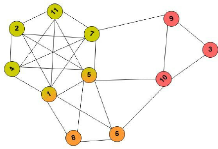
Given this graph, you immediately see a large clique (a fully connected subgraph, nodes 1, 2, 4, 5, 7, 11), that you would instinctively replace with a single measurement right away. You’d continue with the remaining cliques (3, 9, 10 and 8, 6), three measurements in total. The order of replacement is key, if by chance you’d join up the nodes 5, 6, 10 first, you’d end up with 4 measurements in total.

Create the graph

Using the networkx package, I created the aforementioned undirected graph.

import networkx as nx

def create_compatibility_graph(obs_hamiltonian):
    """Create a graph, where the nodes represent measurements and edges are formed for combinable measurments.

    Args:
        - obs_hamiltonian (list(list(str))): List of measurements (list of list of Pauli operators), e.g., [["Y", "I", "Z", "I"], ["Y", "Y", "X", "I"]].

    Returns:
        - (networkx.Graph): graph that represents the measurments and possible combinations thereof
    """
    G = nx.Graph()
    G.add_nodes_from(range(len(obs_hamiltonian)))
    
    for i in range(len(obs_hamiltonian)):
        for j in range(i):
            if check_simplification(obs_hamiltonian[i], obs_hamiltonian[j]):
                G.add_edge(i, j)
    return G

Create the optimizer

Iteratively replace cliques through combined measurements, starting from the biggest clique.

def optimize_measurement_cliques(obs_hamiltonian):
    """Create an optimized (smaller) list of measurements, based on cliques of combinable measurements. 
    Creates a graph representation of the measurements and iteratively combines cliques of measurements,
    starting from the largest.

    Args:
        - obs_hamiltonian (list(list(str))): List of measurements (list of list of Pauli operators), e.g., [["Y", "I", "Z", "I"], ["Y", "Y", "X", "I"]].

    Returns:
        - list(list(str)): an optimized list of measurements
    """
    G = create_compatibility_graph(obs_hamiltonian)
    
    result = []
    
    while True:
        cliques = nx.find_cliques(G) # TODO: this should be done only once

        cliques_list = list(cliques)
        cliques_list.sort(key=len, reverse=True)

        if not cliques_list: # no cliques left
            break
        elif len(cliques_list[0]) == 1: # only singleton cliques left
            result += [list(obs_hamiltonian[c[0]]) for c in cliques_list]
            break
        else: # optimize 
            measurement = optimize_measurements(obs_hamiltonian[cliques_list[0]])
            result += measurement
            G.remove_nodes_from(cliques_list[0])
    
    return result

Test and compare the optimizers

A small routine to create some test data,…

import numpy as np

def create_measurements(count, width):
    """Create ´count´ random measurement sequences of width ´width´.

    Args:
        - count (int): number of random measurements to create
        - width (int): number of Pauli operators per measurement

    Returns:
        - list(list(str)): list of measurements, e.g., [["Y", "I", "Z", "I"], ["Y", "Y", "X", "I"]].
    """
    paulis = np.array(['I', 'X', 'Y', 'Z'])
    
    rand = np.random.randint(0, 4, [count, width], dtype=int)
    return paulis[rand]

Running a few samples..

for width in range(3, 9):
    n_measurements = 3**width # there are up to 4**width possible distinct measurements
    data = create_measurements(n_measurements, width)
    benchmark = optimize_measurements(data)
    cliques = optimize_measurement_cliques(data)
    
    print(width, n_measurements, len(benchmark), len(cliques))

The results show a small, but measurable compression improvement on the initial greedy algorithm.

widthNN (G.O.)N (C.O.)1 – N (C.O.)/N (G.O.)
32712100.166
48132300.063
524383820.012
67292162090.032
721876085830.041
86561167215640.065
The number of measurements N could be reduced with both the greedy optimizer (G.O.) and the clique optimizer (C.O.) significantly. The clique optimizer improved on the greedy optimizer in our test in the range of a few percent points.

QHack 2023: 4 week prep challenge, day 1, The first rule of Quantum Chemistry

I want to attend this years QHack hackathon by Xanadu. To get most out of my experience, I want to shape up, prior to the event. Starting today, I’m committing myself to a 4 week prep challenge. Every day, I will complete some quantum coding exercise, riddle or challenge, I’ll refine my road-map along the way, as a starting point, I’ll take on last years challenges.

Quantum Chemistry: particle conservation (difficulty easy)

The problem statement an base code was taken from this link. It is a rather simple problem, not requiring any particular knowledge in Pennylane, Quantum mechanics or quantum computing beyond a grasp of quantum state representations.

Intro

Larger quantum systems are more conveniently described in second quantization, i.e. a systems state is described by the occupation of a given quantum state (orbital).

Looking at a single molecule, during chemical processes the number of electrons are conserved – none disappear, nor appear out of thin air. If you want to map a molecular Hamiltonian to a qubit Hamiltonian, the used quantum gates need to preserve this particle count. How to mathematically construct suitable operators using the Jordan-Wigner representation is nicely described here. Now a detailed outline on how the problem was solved.

Representation wrangling

Firstly, it comes in handy to convert integer state representations (easy to enumerate) to a second quantization representation of a fixed width (easy to obtain particle counts).

def binary_list(m, n):
    """Converts number m to binary encoded on a list of length n

    Args:
        - m (int): Number to convert to binary
        - n (int): Number of wires in the circuit

    Returns:
        - (list(int)): Binary stored as a list of length n
    """

    bin_str = np.binary_repr(m, width=n)
    arr = [int(s) for s in bin_str]

    return arr

Listing up all basis states of a fixed width

Secondly, all basis states were needed, to test if they were particle conserving under a given quantum circuit.

def basis_states(n):
    """Given a number n, returns a list of all binary_list(m,n) for m < 2**n, thus providing all basis states
         for a circuit of n wires

    Args:
        - n(int): integer representing the number of wires in the circuit

    Returns:
        - (list(list(int))): list of basis states represented as lists of 0s and 1s.
    """

    arr = []
    for m in range(2**n):
        arr += [binary_list(m, n), ]

    return arr

Check if particle conservation is given for a given circuit

Lastly, given a certain width, we obtain the particle counts of all possible state configurations given a certain width. Then we apply a given circuit onto all basis states, and check if the resulting states comprises states with the original particle count. If this is not the case, we abort the test.

def is_particle_preserving(circuit, n):
    """Given a circuit and its number of wires n, returns 1 if it preserves the number of particles, and 0 if it does not

    Args:
        - circuit (qml.QNode): A QNode that has a state such as [0,0,1,0] as an input and outputs the final state after performing
        quantum operation
        - n (int): the number of wires of circuit

    Returns:
        - (bool): True / False according to whether the input circuit preserves the number of particles or not
    """

    particle_counts_in_states = np.array([sum(binary_list(m, n)) for m in range(2**n)])
    
    is_particle_preserving = True
    
    for inp_state in basis_states(n):
        out_state = circuit(inp_state)
        out_contains_base_state = [not np.isclose(base_state, 0.) for base_state in out_state]
        
        if not np.all(particle_counts_in_states[out_contains_base_state] == sum(inp_state)):
            is_particle_preserving = False
            break

    return is_particle_preserving

Test data

The puzzle creators provided two circuits for testing the algorithm.

The first circuit contains the well-known Hadamard and CNOT gates, extensively used for logical operations in quantum computing. Unsurprisingly, these gates are not explicitly designed to fulfill particle conservation, and thus fail our test.

The second circuit contains specially designed DoubleExcitation and SingleExcitation operators, these do fulfill our particle conservation requirement.