QHack 2023: 4 week prep challenge, day 12, Quantum Counting

I continued on the quantum algorithms track, with the quantum counting exercise. The number of solutions to a search problem should be estimated using Grover search and Quantum Phase Estimation.

I’ve found a very concise and clear video on Grover’s algorithm and the accompanying basic example code.

The coding itself boiled down to some basic numpy matrix wrangling, and implementing the proposed algorithm. A more detailed description of the solution scheme can be found here.

Since I had a little more time, I also read up on QFT arithmetics. I wasn’t aware of the tutorial yesterday, it would have been very helpful though!

QHack 2023: 4 week prep challenge, day 11, A Quantum Adder (QFT)

Today, I’m continuing with the next exercise from the algorithms track. The task is to build a number adder using the Fourier space.

Firstly, a Fourier transform is applied on the initial state, i.e. a state |0> or |1> in the computational basis is flipped into the X-Y-plane. The qubits are then rotated around the Z-axis, with an angle according to the number to add. Eventually, the state is transformed back from the Fourier space.

The transformation rule for the QFT reads

\[ QFT|x\rangle = \frac{1}{\sqrt{M}} \sum^{M-1}_{k=0} \exp(\frac{2 \pi i}{M} x k) |k\rangle \]

If you now want to add to a state in the Fourier space, you have to rotate the qubits accordingly. It is important to notice, that a rotation only effects the |1> portion, but not the |0> portion of a qubit’s state.

Having that in mind, it was relatively straight forward to come up with the solution…

def qfunc_adder(m, wires):
    """Quantum function capable of adding m units to a basic state given as input.

    Args:
        - m (int): units to add.
        - wires (list(int)): list of wires in which the function will be executed on.
    """

    qml.QFT(wires=wires)

    for w, _ in enumerate(wires):
        angle = m*np.pi/(2**w)
        qml.RZ(angle, wires=w)

    qml.QFT(wires=wires).inv()

… the tests check out, success!

QHack 2023: 4 week prep challenge, day 10, A topology survey

I continued on the Algorithm track with the adapting topologies exercise. It is an easy, but very enjoyable task, I just really like working with graphs.

Topology

Quanta need to be next to each other, when performing multi-qubit operations like CNOT, SWAP, etc. on them. If you want to perform a multi-qubit operation on non-adjacent qubits, you’ve got to SWAP them around, until they are next to each other. Therefore, a higher connectivity is beneficial to save up coherence for the main calculations.

However, operations on qubits may cause cross-talk on neighboring qubits, and therefore reducing coherence.

Now the topology of a QPU has to weigh-in both effects, and there are topologies that optimize for reduced cross-talk (e.g. ion traps), maximal connectivity, or seek to balance the two (e.g. IBM’s heavy hexagonal lattice).

Exercise

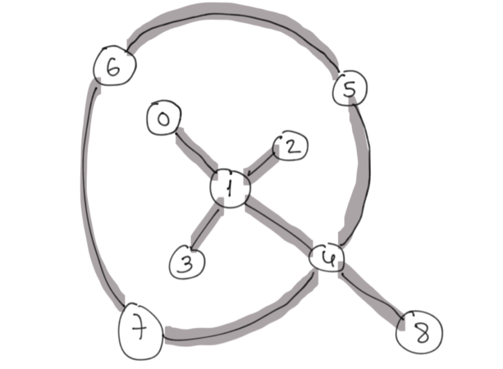
Now in this exercise, a toy topology is provided, and the challenge is to calculate the number of SWAPs required to perform a CNOT gate. For this, I used the python library networkx.

Toy topology, taken from here.
import networkx as nx

def get_topology_graph():
    """Create an adjacency graph, of the topology dict.
    
    Args:
    
    Returns: 
        - (nx.Graph): adjacency graph
    """
    
    G = nx.Graph()
    
    for i, nodes in graph.items():
        elist = [(i, j) for j in nodes]
        G.add_edges_from(elist)
    
    return G

The SWAP count, is then easily calculated from the length of the shortest path (don’t forget to rewind the operations, to clean up after the CNOT).

def n_swaps(cnot):
    """Count the minimum number of swaps needed to create the equivalent CNOT.

    Args:
        - cnot (qml.Operation): A CNOT gate that needs to be implemented on the hardware
        You can find out the wires on which an operator works by asking for the 'wires' attribute: 'cnot.wires'

    Returns:
        - (int): minimum number of swaps
    """
    
    G = get_topology_graph()
    wires = cnot.wires
    path = nx.shortest_path(G, wires[0], wires[1])
    
    return 2*(len(path)-2)

The results check out, success!

Plotting a sample circuit

To round the story up, I wrote a small routine to build out a circuit, that actually swaps the qubits around ..

dev = qml.device("default.qubit", wires=len(graph))

@qml.qnode(dev)
def n_swaps_perf(wire1, wire2):
    G = get_topology_graph()
    
    path = nx.shortest_path(G, wire1, wire2)
    path.pop(-1) # remove last item, to have easier indexing in loops
    
    for i in range(1, len(path)):
        qml.SWAP(wires=[path[i], path[i-1]])
        
    qml.CNOT(wires=[path[-1], wire2])
    
    rev_path = list(reversed(path))
    
    for i in range(1, len(rev_path)):
        qml.SWAP(wires=[rev_path[i], rev_path[i-1]])
        
    return qml.expval(qml.PauliZ(wires=wire2))

.. and plots the resulting circuit.

drawer = qml.draw(n_swaps_perf)
print(drawer(8,2))
1: ───────╭SWAP─╭●─╭SWAP───────┤     
2: ───────│────╰X─│───────────┤  <Z>
4: ─╭SWAP─-╰SWAP────╰SWAP─╭SWAP─-┤     
8: ─╰SWAP────────────────╰SWAP─┤     

Looks good.

QHack 2023: 4 week prep challenge, day 9, Deutsch Jozsa algorithm

Today is a very tired day, I just solved the easiest puzzle from the Algorithms track to keep the rhythm. Deutsch Josza algorithm.
Meanwhile, I registered for the iQuHack event this weekend. It is organized by people associated with the MIT and Microsoft is a sponsor of the remote-track. I plan to take a look through resources from the previous years, and probably a few Q# resources to have a rough idea what is awaiting me, and possibly have a more enjoyable experience.

QHack 2023: 4 week prep challenge, day 8, Pennylane 101

I’m struggling with the next exercise (Who likes the beatles, k-NN) on the ML track, I will have to read up on embeddings and the swap test. My web search lead me to this Pennylane forum entry, but the proposed solution looks not quite right to me. Well, after some coding and some tests, I decided I was too tired to do the harder reading and opted to solidify some concepts and solve a few easier exercises instead. On the Pennylane 101-track, I solved the exercises 1, 2, 3, and 4. Following, are a few thoughts I had along the way…

Ad Exercise 1, gate order

The exercise highlighted the non-commuting nature of operators.

Ad Exercise 2, devices

Pennylane offers multiple (simulation) devices to choose from, a brief listing

  • default device
  • devices to use in combination with ML frameworks (JAX, PyTorch, TensorFlow)
  • device for mixed state calculations
  • device for Quitrits. Quitrits enable calculations in a three-valued logic, there may be some physical advantages to such systems (stability, …), but I picture quite some mental gymnastics to deal with them.

Ad Exercise 3, superdense coding

With super dense coding, it is possible to send 2-bits of information, while transmitting only one qubit after defining the message (One entangled qubit without information is sent before defining the message).

To solve the exercise, I used a RY gate to emulate a noisy Hadamard gate.

Interesting to me, was the qml.broadcast command, that offers a number of handy wiring patterns, and will spare me a few loops in the future.

Ad Exercise 4, finite difference method

For VQE optimizations, it is essential to have the gradients of a given circuit. Differentiability is generally a very important aspect of the Pennylane library. It is worthwhile to recap the different differentiation methods:

  • backprop
  • adjoint
  • parameter-shift
  • finite-diff

These options also enter my reading list.

QHack 2023: 4 week prep challenge, day 7, VQE

I am continuing my preparations, following the QHack 2022 challenges. I’ll tackle the QML track, again starting from the most basic example, I am trying to solve them correctly, and learn as much as I can along the way.

Knowing a field, always requires the knowledge of it’s language. I recall the days in my physics studies, where different branches used different words of the same entities – it gave me a really hard time. Interesting are also the cases where you are using a “default” option, out of many possible options, and are surprised when someone diligently states the choice explicitly: Most calculations in quantum computing are performed in the computational basis, i.e. the eigenbasis of the Pauli-Z operator

\[ \sigma_z = \left(\begin{array}{rrr} 1 & 0 \\ 0 & -1 \end{array}\right) \]

A notable alternative is the Fourier basis. Goal of this exercise, will be to approximate the Fourier transform of a given state in the computational basis, using a VQE routine.

Approximate the QFT of a state

To solve this exercise, it is sufficient to implement the pre-sketched ansatz, and a cost function.

@qml.qnode(dev)
def circuit(angles):
    """This is the quantum circuit that we will use."""
     # Add the template of the statement with the angles passed as an argument.
    for i, angle in enumerate(angles):
        qml.Hadamard(wires=i)
        qml.RZ(angle, wires=i)

    # We apply QFT^-1 to return to the computational basis.
    # This will help us to see how well we have done.
    qml.adjoint(qml.QFT)(wires=range(n_qubits))

    # We return the probabilities of seeing each basis state.
    return qml.probs(wires=range(n_qubits))

def error(angles):
    """This function will determine, given a set of angles, how well it approximates
    the desired state. Here it will be necessary to call the circuit to work with these results.
    """

    probs = circuit(angles)
        
    # The return error should be smaller when the state m is more likely to be obtained.
    return 1-probs[m]

The tests check out, a very simple exercise.

This task is mostly academic, there is a general algorithm to perform the QFT and the solution puts much computational effort in finding the FT of a single state. However, I used my daily time budget to get a quick refresher on the QFT and it’s usages, as well as to do some exploratory reading. So it was again a productive day.

QHack 2023: 4 week prep challenge, day 6, H-H first excited state

Almost a week passed, it’s time for more tricky tasks! The last and most advanced exercise in the Quantum Chemistry track of the 2022 QHack.

Disclaimer: At the time being, the proposed solution does not produce the correct results.

The task is to obtain the energy of the first excited state of an H-H molecule at a given nuclei distance. This is achieved by firstly calculating the ground state energy, and later modifying the systems Hamiltonian to penalize the actual ground state. Repeating the ground-state calculation with the modified Hamiltonian, you can obtain the first excited state.

The calculation of the ground-state via a VQE routine, is done following the concise Pennylane VQE tutorial, with only minuscule modifications.

import sys
import pennylane as qml
from pennylane import numpy as np
from pennylane import hf


def ground_state_VQE(H):
    """Perform VQE to find the ground state of the H2 Hamiltonian.

    Args:
        - H (qml.Hamiltonian): The Hydrogen (H2) Hamiltonian

    Returns:
        - (float): The ground state energy
        - (np.ndarray): The ground state calculated through your optimization routine
    """

    qubits = 4
    
    dev = qml.device("default.qubit", wires=qubits)
    
    electrons = 2
    hf = qml.qchem.hf_state(electrons, qubits)
    
    def circuit(param, wires):
        qml.BasisState(hf, wires=wires)
        qml.DoubleExcitation(param, wires=range(qubits))
    
    @qml.qnode(dev)
    def cost_fn(param):
        circuit(param, wires=range(qubits))
        return qml.expval(H)
    
    @qml.qnode(dev)
    def ground_state(param, wires):
        circuit(param, wires)
        return qml.state()
    
    opt = qml.GradientDescentOptimizer(stepsize=0.1)
    theta = np.array(0.0, requires_grad=True)
    
    # store the values of the cost function
    energy = [cost_fn(theta)]

    # store the values of the circuit parameter
    angle = [theta]

    max_iterations = 100
    conv_tol = 1e-06

    for n in range(max_iterations):
        theta, prev_energy = opt.step_and_cost(cost_fn, theta)

        energy.append(cost_fn(theta))
        angle.append(theta)

        conv = np.abs(energy[-1] - prev_energy)

        if n % 2 == 0:
            print(f"Step = {n},  Energy = {energy[-1]:.8f} Ha, theta = {theta:.3f}")

        if conv <= conv_tol:
            break

    E0 = energy[-1]
    gstate = ground_state(theta, wires=range(qubits))
    
    return E0, gstate

symbols = ["H", "H"]
coord = 0.6614
geometry = np.array([[0.0, 0.0, -coord], [0.0, 0.0, coord]], requires_grad=False)
mol = hf.Molecule(symbols, geometry)

H = hf.generate_hamiltonian(mol)()
E0, ground_state = ground_state_VQE(H)

The next step is to calculate a modified Hamiltonian.

def create_H1(ground_state, beta, H):
    """Create the H1 matrix, then use `qml.Hermitian(matrix)` to return an observable-form of H1.

    Args:
        - ground_state (np.ndarray): from the ground state VQE calculation
        - beta (float): the prefactor for the ground state projector term
        - H (qml.Hamiltonian): the result of hf.generate_hamiltonian(mol)()

    Returns:
        - (qml.Observable): The result of qml.Hermitian(H1_matrix)
    """

    H1 = qml.matrix(H) + beta * np.outer(ground_state, ground_state)
    qubits = int(np.log2(len(ground_state)))
    return qml.Hermitian(H1, wires=range(qubits))


def excited_state_VQE(H1):
    """Perform VQE using the "excited state" Hamiltonian.

    Args:
        - H1 (qml.Observable): result of create_H1

    Returns:
        - (float): The excited state energy
    """

    E1, estate = ground_state_VQE(H1)
    return E1

beta = 15.0
H1 = create_H1(ground_state, beta, H)
E1 = excited_state_VQE(H1)

print(E1)

While the ground state energy is correctly calculated, some error remains in the calculation of the excited state energy (larger than zero). … I will leave it to rest for the next few days, and maybe revisit it later.

QHack 2023: 4 week prep challenge, day 5, Triple excitation Givens rotation

Continuing on the Quantum Chemistry track, the next exercise. According to the designers, it is more difficult than the last ones, but it suited me very well. With the knowledge of the previous days, I could solve the task by merely looking at it.

The task is to prepare the state

\[ |\psi(\alpha, \beta, \gamma)\rangle = \cos{\frac{\alpha}{2}} \cos{\frac{\beta}{2}} \left[ \cos{\frac{\gamma}{2}} |111000\rangle – \sin{\frac{\gamma}{2}}|000111\rangle \right] – \cos{\frac{\alpha}{2}} \sin{\frac{\beta}{2}}|001011\rangle – \sin{\frac{\alpha}{2}} |011001\rangle \]

using a single excitation, a double excitation and a triple excitation, the latter one should be constructed from a matrix.

Constructing a triple excitation Givens rotation

This is a really straight forward task. The transformation rules are analogous to the single and double excitations

\[ G^{(3)}(\gamma)|000111\rangle = \cos{\frac{\gamma}{2}} | 000111\rangle + \sin{\frac{\gamma}{2}} |111000\rangle \\ G^{(3)}(\gamma)|111000\rangle = \cos{\frac{\gamma}{2}} | 111000\rangle – \sin{\frac{\gamma}{2}} |000111\rangle \]

and the realization, that the decimal representations of the states provide you with the target indices in the transformation matrix

\[ |000111\rangle = |7\rangle, \\ |111000\rangle = |56\rangle \]

yields the implementation

def triple_excitation_matrix(gamma):
    """The matrix representation of a triple-excitation Givens rotation.
https://github.com/XanaduAI/QHack2022/tree/master/Coding_Challenges/qchem_400_TripleGivens_template 
    Args:
        - gamma (float): The angle of rotation

    Returns:
        - (np.ndarray): The matrix representation of a triple-excitation
    """

    dim = 2**6
    res = np.identity(dim)
    
    # |000111> = |7>
    # G3(theta)|7> = cos(theta/2)|7> + sin(theta/2)|56>
    row7 = np.zeros(dim)
    row7[7] = np.cos(gamma/2)
    row7[56] = -np.sin(gamma/2)
    
    # |111000> = |56>
    # G3(theta)|56> = cos(theta/2)|56> - sin(theta/2)|7>
    row56 = np.zeros(dim)
    row56[7] = np.sin(gamma/2)
    row56[56] = np.cos(gamma/2)
    
    res[7] = row7
    res[56] = row56
    
    return res

Preparing the target state

This was solved by looking at the states and the pre-factors. The basis-states with a single pre-factor underwent only a single Givens rotation…

@qml.qnode(dev)
def circuit(angles):
    """Prepares the quantum state in the problem statement and returns qml.probs

    Args:
        - angles (list(float)): The relevant angles in the problem statement in this order:
        [alpha, beta, gamma]

    Returns:
        - (np.tensor): The probability of each computational basis state
    """

    # QHACK #
    qml.BasisState(np.array([1, 1, 1, 0, 0, 0]), wires=[0, 1, 2, 3, 4, 5])
    qml.SingleExcitation(angles[0], wires=[0, 5])
    qml.DoubleExcitation(angles[1], wires=[0,1,4,5])
    qml.QubitUnitary(triple_excitation_matrix(angles[2]), wires=[0,1,2,3,4,5])
    # QHACK #

    return qml.probs(wires=range(NUM_WIRES))

The provided test datasets yield the correct results, success!

QHack 2023: 4 week prep challenge, day 1, The first rule of Quantum Chemistry

I want to attend this years QHack hackathon by Xanadu. To get most out of my experience, I want to shape up, prior to the event. Starting today, I’m committing myself to a 4 week prep challenge. Every day, I will complete some quantum coding exercise, riddle or challenge, I’ll refine my road-map along the way, as a starting point, I’ll take on last years challenges.

Quantum Chemistry: particle conservation (difficulty easy)

The problem statement an base code was taken from this link. It is a rather simple problem, not requiring any particular knowledge in Pennylane, Quantum mechanics or quantum computing beyond a grasp of quantum state representations.

Intro

Larger quantum systems are more conveniently described in second quantization, i.e. a systems state is described by the occupation of a given quantum state (orbital).

Looking at a single molecule, during chemical processes the number of electrons are conserved – none disappear, nor appear out of thin air. If you want to map a molecular Hamiltonian to a qubit Hamiltonian, the used quantum gates need to preserve this particle count. How to mathematically construct suitable operators using the Jordan-Wigner representation is nicely described here. Now a detailed outline on how the problem was solved.

Representation wrangling

Firstly, it comes in handy to convert integer state representations (easy to enumerate) to a second quantization representation of a fixed width (easy to obtain particle counts).

def binary_list(m, n):
    """Converts number m to binary encoded on a list of length n

    Args:
        - m (int): Number to convert to binary
        - n (int): Number of wires in the circuit

    Returns:
        - (list(int)): Binary stored as a list of length n
    """

    bin_str = np.binary_repr(m, width=n)
    arr = [int(s) for s in bin_str]

    return arr

Listing up all basis states of a fixed width

Secondly, all basis states were needed, to test if they were particle conserving under a given quantum circuit.

def basis_states(n):
    """Given a number n, returns a list of all binary_list(m,n) for m < 2**n, thus providing all basis states
         for a circuit of n wires

    Args:
        - n(int): integer representing the number of wires in the circuit

    Returns:
        - (list(list(int))): list of basis states represented as lists of 0s and 1s.
    """

    arr = []
    for m in range(2**n):
        arr += [binary_list(m, n), ]

    return arr

Check if particle conservation is given for a given circuit

Lastly, given a certain width, we obtain the particle counts of all possible state configurations given a certain width. Then we apply a given circuit onto all basis states, and check if the resulting states comprises states with the original particle count. If this is not the case, we abort the test.

def is_particle_preserving(circuit, n):
    """Given a circuit and its number of wires n, returns 1 if it preserves the number of particles, and 0 if it does not

    Args:
        - circuit (qml.QNode): A QNode that has a state such as [0,0,1,0] as an input and outputs the final state after performing
        quantum operation
        - n (int): the number of wires of circuit

    Returns:
        - (bool): True / False according to whether the input circuit preserves the number of particles or not
    """

    particle_counts_in_states = np.array([sum(binary_list(m, n)) for m in range(2**n)])
    
    is_particle_preserving = True
    
    for inp_state in basis_states(n):
        out_state = circuit(inp_state)
        out_contains_base_state = [not np.isclose(base_state, 0.) for base_state in out_state]
        
        if not np.all(particle_counts_in_states[out_contains_base_state] == sum(inp_state)):
            is_particle_preserving = False
            break

    return is_particle_preserving

Test data

The puzzle creators provided two circuits for testing the algorithm.

The first circuit contains the well-known Hadamard and CNOT gates, extensively used for logical operations in quantum computing. Unsurprisingly, these gates are not explicitly designed to fulfill particle conservation, and thus fail our test.

The second circuit contains specially designed DoubleExcitation and SingleExcitation operators, these do fulfill our particle conservation requirement.