QHack 2023: 4 week prep-challenge, day 18, QAOA with custom Hamiltonian

The final exercise on the QML track, included some bug-hunting for me, but this made it much more rewarding, to eventually solve it.

The basic task was conceivably easy: given some data, create a hamiltonian and use a QAOA optimization scheme to obtain a ground state approximation. The problem described some special graph covering problem. The mistakes that took some efforts to resolve where

  • Mistake 1: PennyLane is exceptionally greedy, when arrays appear along the optimization scheme. The way I constructed the hamiltonian included numpy arrays for indexing qubits, PennyLane tried to differentiate the problem by them and vary them subsequently – that lead to exceptions, and it was a real pain to find the source of the error.
  • Mistake 2: I tried to construct operators, instead of decomposing the occupation operator into Pauli matrices. This might work somehow, but I had an easier time decomposing the operators eventually.
  • Mistake 3: I omitted the constant terms, the optimal configuration is not affected by the constant term, but my tests relied on the final energy.

The code for the Hamiltonian

def hamiltonian_coeffs_and_obs(graph):
    """Creates an ordered list of coefficients and observables used to construct
    the UDMIS Hamiltonian.

    Args:
        - graph (list((float, float))): A list of x,y coordinates. e.g. graph = [(1.0, 1.1), (4.5, 3.1)]

    Returns:
        - coeffs (list): List of coefficients for elementary parts of the UDMIS Hamiltonian
        - obs (list(qml.ops)): List of qml.ops
    """

    num_vertices = len(graph)
    E, num_edges = edges(graph)
    u = 1.35
    obs = []
    coeffs = []

    # single terms
    for i in range(num_vertices):
        obs.append(qml.PauliZ(wires=i))
        coeffs.append(-.5)
    
    # constant term
    obs.append(qml.Identity(wires=0))
    coeffs.append(-.5*num_vertices)
    
    # interaction terms
    pairs = np.argwhere(E>0)
    for pair in pairs:
        i = int(pair[0])
        j = int(pair[1])
        obs.append(qml.PauliZ(wires=i) @ qml.PauliZ(wires=j))
        coeffs.append(.25*u)
        coeffs[i] += .25*u
        coeffs[j] += .25*u
        coeffs[num_vertices] += .25*u
    
    return coeffs, obs

The tests check out, success!

QHack 2023: 4 week prep challenge, day 16, Variational Quantum Classifier

I continued with the next exercise on the QML track, the task was to create a VQC (Variational Quantum Classifier) to classify Ising-spin systems into ordered and disordered states, with an accuracy of at least 90%.

The Ising model, is a simplified model of a ferromagnet, describing it’s magnetic properties. A ferromagnet displays spontaneous magnetization (i.e. parallel alignment of it’s atoms spins) below its critical temperature. In our dataset, the ferromagnet is represented by five spins arranged in a linear setup.

Variational Quantum Classifier

A Variational Quantum Classifier differs in two essential points from a conventional NN classifier. Firstly, the input data needs to be encoded into qubits. Secondly, the hypothesis function is a parameterized quantum circuit. These parameters are subsequently optimized using classical optimizers.

Implementation

My implementation heavily draws on the PennyLane VQC tutorial, I made a few adaption though.

First we need to create our hypothesis, similarly to the tutorial I chose strongly entangling layers. I only want to distinguish two classes, and I do not want to create a quantum-classical hybrid pipeline (apart from the classically added bias term). Therefore, I only need the expectation value of a single qubit, it doesn’t matter which one I choose.

@qml.qnode(dev)
def circuit(weights, x):
    """VQC architecture, encodes input data and performs a series of strongly entangling layers, to perform the classification.
    
    Args:
        - weights (np.ndarray): weights for the entangling layers
        - x (np.ndarray): spin configurations

    Returns:
        - prediction (float): expectation value of one qubit, after the entangling layers
    """
    qml.BasisState(x, wires=range(num_wires))
    qml.StronglyEntanglingLayers(weights=weights, wires=range(4))

    return qml.expval(qml.PauliZ(0))

def variational_classifier(weights, bias, x):
    return circuit(weights, x) + bias

Next, I initialize my parameters and my optimizer. I opted for three layers, and a smaller step size.

np.random.seed(0)
n_layers = 3
shape = qml.StronglyEntanglingLayers.shape(n_layers=n_layers, n_wires=num_wires)
weights = np.random.random(size=shape)
bias = np.array(0.0, requires_grad=True)
    
opt = NesterovMomentumOptimizer(0.1)
batch_size = 10

Finally, the optimization loop …

for it in range(25):

    # Update the weights by one optimizer step
    batch_index = np.random.randint(0, len(ising_configs), (batch_size,))
    X_batch = ising_configs[batch_index]
    Y_batch = labels[batch_index]
    weights, bias, _, _ = opt.step(cost, weights, bias, X_batch, Y_batch)

    # Compute accuracy
    predictions = [np.sign(variational_classifier(weights, bias, x)) for x in ising_configs]
    acc = accuracy(labels, predictions)

    print(
        "Iter: {:5d} | Cost: {:0.7f} | Accuracy: {:0.7f} ".format(
            it + 1, cost(weights, bias, ising_configs, labels), acc
        )
    )

I reach an accuracy of 93.6%, a good result for this toy problem.

QHack 2023: 4 week prep challenge, day 15, SWAP Test

I did another basic exercise on the QML track, but honestly, I was struggling a lot with this one. The hard-earned victories are both satisfying and instructive. But first a quick outline of the exercise.

The challenge was to estimate the inner product of two feature vectors. A distance measure is derived from this quantity and is used to perform a k-NN (k-nearest neighbor) algorithm – in this configuration an artificial use case.

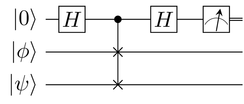
The inner product can be estimated with the SWAP-test.

SWAP test circuit, taken from Wikipedia.

The inner product estimate is calculated from

\[ P(\text{control qubit} = 0) = \frac{1}{2} + \frac{1}{2}\lvert\langle \psi | \phi \rangle\rvert^2 \]

Implementation

In this implementation, each feature vector is normalized, and since each vector has dimension two, a single qubit suffices to encode the data.

from pennylane import numpy as np
import pennylane as qml


def distance(A, B):
    """Function that returns the distance between two vectors.

    Args:
        - A (list[int]): person's information: [age, minutes spent watching TV].
        - B (list[int]): person's information: [age, minutes spent watching TV].

    Returns:
        - (float): distance between the two feature vectors.
    """

    def prep_state():
        """Function that encodes the two 2D feature vectors into the amplitudes of one qubit each."""
        
        tan_thetaA = A[0]/A[1]
        thetaA = np.arctan(tan_thetaA)
        tan_thetaB = B[0]/B[1]
        thetaB = np.arctan(tan_thetaB)
        
        qml.RY(2.*thetaA, wires=0)
        qml.RY(2.*thetaB, wires=1)
    
    
    dev = qml.device("default.qubit", wires=3)
    @qml.qnode(dev)
    def circuit():
        """Quantum circuit that encodes two 2D-feature vectors and performs a SWAP test.
        
        Returns:
            - ([float, float]): probabilities of states measured on the control qubit.
        """
        prep_state()
        
        qml.Hadamard(wires=2)
        qml.CSWAP(wires=range(2,-1,-1))
        qml.Hadamard(wires=2)
        
        return qml.probs(2)

    # print(qml.draw(circuit)())
    
    tmp = circuit()[0] # .5 + .5<A,B>^2
    A_times_B = np.sqrt(2.*tmp-1.)
    
    return np.sqrt(2*(1.-A_times_B))

The provided tests check out.

Lessons learned

I will seize this opportunity to reflect upon my solution strategies. The problem statement was a little less concrete than the ones of previous exercises. In the starter code two hints were pointing at the SWAP Test and the PennyLane amplitude encoding functionality. After an initial implementation failed, I did some more research and found a SWAP-test implementation on a PennyLane forum. This was more confusing then helpful, I believe the core confusion being how the normalization is done in this encoding strategy.

Anyways, the clean bottom up solution, along with some debugging print-outs eventually worked out.