QHack 2023: 4 week prep challenge, day 6, H-H first excited state

Almost a week passed, it’s time for more tricky tasks! The last and most advanced exercise in the Quantum Chemistry track of the 2022 QHack.

Disclaimer: At the time being, the proposed solution does not produce the correct results.

The task is to obtain the energy of the first excited state of an H-H molecule at a given nuclei distance. This is achieved by firstly calculating the ground state energy, and later modifying the systems Hamiltonian to penalize the actual ground state. Repeating the ground-state calculation with the modified Hamiltonian, you can obtain the first excited state.

The calculation of the ground-state via a VQE routine, is done following the concise Pennylane VQE tutorial, with only minuscule modifications.

import sys
import pennylane as qml
from pennylane import numpy as np
from pennylane import hf


def ground_state_VQE(H):
    """Perform VQE to find the ground state of the H2 Hamiltonian.

    Args:
        - H (qml.Hamiltonian): The Hydrogen (H2) Hamiltonian

    Returns:
        - (float): The ground state energy
        - (np.ndarray): The ground state calculated through your optimization routine
    """

    qubits = 4
    
    dev = qml.device("default.qubit", wires=qubits)
    
    electrons = 2
    hf = qml.qchem.hf_state(electrons, qubits)
    
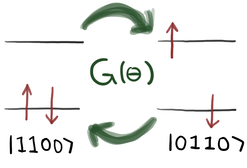
    def circuit(param, wires):
        qml.BasisState(hf, wires=wires)
        qml.DoubleExcitation(param, wires=range(qubits))
    
    @qml.qnode(dev)
    def cost_fn(param):
        circuit(param, wires=range(qubits))
        return qml.expval(H)
    
    @qml.qnode(dev)
    def ground_state(param, wires):
        circuit(param, wires)
        return qml.state()
    
    opt = qml.GradientDescentOptimizer(stepsize=0.1)
    theta = np.array(0.0, requires_grad=True)
    
    # store the values of the cost function
    energy = [cost_fn(theta)]

    # store the values of the circuit parameter
    angle = [theta]

    max_iterations = 100
    conv_tol = 1e-06

    for n in range(max_iterations):
        theta, prev_energy = opt.step_and_cost(cost_fn, theta)

        energy.append(cost_fn(theta))
        angle.append(theta)

        conv = np.abs(energy[-1] - prev_energy)

        if n % 2 == 0:
            print(f"Step = {n},  Energy = {energy[-1]:.8f} Ha, theta = {theta:.3f}")

        if conv <= conv_tol:
            break

    E0 = energy[-1]
    gstate = ground_state(theta, wires=range(qubits))
    
    return E0, gstate

symbols = ["H", "H"]
coord = 0.6614
geometry = np.array([[0.0, 0.0, -coord], [0.0, 0.0, coord]], requires_grad=False)
mol = hf.Molecule(symbols, geometry)

H = hf.generate_hamiltonian(mol)()
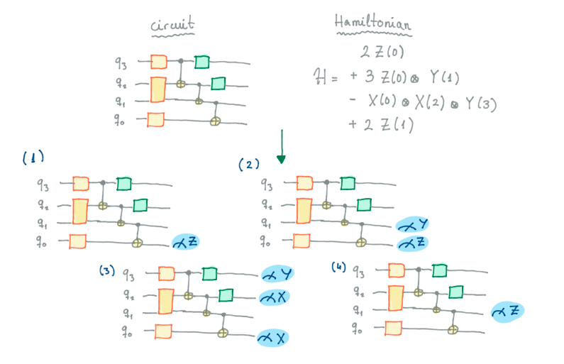
E0, ground_state = ground_state_VQE(H)

The next step is to calculate a modified Hamiltonian.

def create_H1(ground_state, beta, H):
    """Create the H1 matrix, then use `qml.Hermitian(matrix)` to return an observable-form of H1.

    Args:
        - ground_state (np.ndarray): from the ground state VQE calculation
        - beta (float): the prefactor for the ground state projector term
        - H (qml.Hamiltonian): the result of hf.generate_hamiltonian(mol)()

    Returns:
        - (qml.Observable): The result of qml.Hermitian(H1_matrix)
    """

    H1 = qml.matrix(H) + beta * np.outer(ground_state, ground_state)
    qubits = int(np.log2(len(ground_state)))
    return qml.Hermitian(H1, wires=range(qubits))


def excited_state_VQE(H1):
    """Perform VQE using the "excited state" Hamiltonian.

    Args:
        - H1 (qml.Observable): result of create_H1

    Returns:
        - (float): The excited state energy
    """

    E1, estate = ground_state_VQE(H1)
    return E1

beta = 15.0
H1 = create_H1(ground_state, beta, H)
E1 = excited_state_VQE(H1)

print(E1)

While the ground state energy is correctly calculated, some error remains in the calculation of the excited state energy (larger than zero). … I will leave it to rest for the next few days, and maybe revisit it later.

QHack 2023: 4 week prep challenge, day 5, Triple excitation Givens rotation

Continuing on the Quantum Chemistry track, the next exercise. According to the designers, it is more difficult than the last ones, but it suited me very well. With the knowledge of the previous days, I could solve the task by merely looking at it.

The task is to prepare the state

\[ |\psi(\alpha, \beta, \gamma)\rangle = \cos{\frac{\alpha}{2}} \cos{\frac{\beta}{2}} \left[ \cos{\frac{\gamma}{2}} |111000\rangle – \sin{\frac{\gamma}{2}}|000111\rangle \right] – \cos{\frac{\alpha}{2}} \sin{\frac{\beta}{2}}|001011\rangle – \sin{\frac{\alpha}{2}} |011001\rangle \]

using a single excitation, a double excitation and a triple excitation, the latter one should be constructed from a matrix.

Constructing a triple excitation Givens rotation

This is a really straight forward task. The transformation rules are analogous to the single and double excitations

\[ G^{(3)}(\gamma)|000111\rangle = \cos{\frac{\gamma}{2}} | 000111\rangle + \sin{\frac{\gamma}{2}} |111000\rangle \\ G^{(3)}(\gamma)|111000\rangle = \cos{\frac{\gamma}{2}} | 111000\rangle – \sin{\frac{\gamma}{2}} |000111\rangle \]

and the realization, that the decimal representations of the states provide you with the target indices in the transformation matrix

\[ |000111\rangle = |7\rangle, \\ |111000\rangle = |56\rangle \]

yields the implementation

def triple_excitation_matrix(gamma):
    """The matrix representation of a triple-excitation Givens rotation.
https://github.com/XanaduAI/QHack2022/tree/master/Coding_Challenges/qchem_400_TripleGivens_template 
    Args:
        - gamma (float): The angle of rotation

    Returns:
        - (np.ndarray): The matrix representation of a triple-excitation
    """

    dim = 2**6
    res = np.identity(dim)
    
    # |000111> = |7>
    # G3(theta)|7> = cos(theta/2)|7> + sin(theta/2)|56>
    row7 = np.zeros(dim)
    row7[7] = np.cos(gamma/2)
    row7[56] = -np.sin(gamma/2)
    
    # |111000> = |56>
    # G3(theta)|56> = cos(theta/2)|56> - sin(theta/2)|7>
    row56 = np.zeros(dim)
    row56[7] = np.sin(gamma/2)
    row56[56] = np.cos(gamma/2)
    
    res[7] = row7
    res[56] = row56
    
    return res

Preparing the target state

This was solved by looking at the states and the pre-factors. The basis-states with a single pre-factor underwent only a single Givens rotation…

@qml.qnode(dev)
def circuit(angles):
    """Prepares the quantum state in the problem statement and returns qml.probs

    Args:
        - angles (list(float)): The relevant angles in the problem statement in this order:
        [alpha, beta, gamma]

    Returns:
        - (np.tensor): The probability of each computational basis state
    """

    # QHACK #
    qml.BasisState(np.array([1, 1, 1, 0, 0, 0]), wires=[0, 1, 2, 3, 4, 5])
    qml.SingleExcitation(angles[0], wires=[0, 5])
    qml.DoubleExcitation(angles[1], wires=[0,1,4,5])
    qml.QubitUnitary(triple_excitation_matrix(angles[2]), wires=[0,1,2,3,4,5])
    # QHACK #

    return qml.probs(wires=range(NUM_WIRES))

The provided test datasets yield the correct results, success!

QHack 2023: 4 week prep challenge, day 4, Givens rotations

Today, I’m heading again for a prepared exercise, the next exercise in the QHack 2022 Quantum Chemistry track. It requires slightly more preparation, than the previous two, but again very doable.

The challenge, invites to get more acquainted with Givens rotations, i.e. operations that allow to transform states, while preserving the hamming weight (the number of ones and zeros). They are the basic building blocks of quantum chemistry and “can be used to construct any kind of particle-conserving circuit”.

The goal is to find the correct rotation angles to transform a start state to a target state, with a quantum circuit with three Givens rotations,

\[|\Psi \rangle = CG^{(1)}(\theta_3; 0,1,3) G^{(2)}(\theta_2; 2,3,4,5) G^{(2)}(\theta_1; 0,1,2,3) |110000\rangle = \\ a |110000\rangle + b |001100 \rangle + c |000011 \rangle + d |100100\rangle \]

Getting to know Givens rotations

Givens rotations, describe transitions of electrons from a starting state to an excited state. In Pennylane, these rotations can be used via the classes qml.SingleExcitation and qml.DoubleExcitation. The linked tutorial is very recommendable.

A Givens rotation can be used to couple states that differ by a single excitation. Image taken from the Xanadu tutorial on Givens rotations.

Solving the exercise

To solve this exercise, I used the rotations’ transformation rules to reach an expression that associated trigonometric functions with the target factors. Further, I used the fact, that states are normalized at any time during the calculation. Key for me to solve it, was to apply only the first two rotations and used the normalization property of the state, from this I obtained the first angle. Then I went on to apply the remaining rotation and easily expressed the missing two angles.

import numpy as np


def givens_rotations(a, b, c, d):
    """Calculates the angles needed for a Givens rotation to out put the state with amplitudes a,b,c and d

    Args:
        - a,b,c,d (float): real numbers which represent the amplitude of the relevant basis states (see problem statement). Assume they are normalized.

    Returns:
        - (list(float)): a list of real numbers ranging in the intervals provided in the challenge statement, which represent the angles in the Givens rotations,
        in order, that must be applied.
    """

    theta1 = 2.*np.arccos(np.sqrt(1-b**2-c**2))
    theta2 = 2.*np.arcsin(c/np.sin(theta1/2.))
    theta3 = 2.*np.arccos(a/np.cos(theta1/2.))
    
    return [theta1, theta2, theta3]

Test

Defining the circuit…

import pennylane as qml

dev = qml.device('default.qubit', wires=6)

@qml.qnode(dev)
def circuit(x, y, z):
    qml.BasisState(np.array([1, 1, 0, 0, 0, 0]), wires=[i for i in range(6)])
    qml.DoubleExcitation(x, wires=[0, 1, 2, 3])
    qml.DoubleExcitation(y, wires=[2, 3, 4, 5])
    # single excitation controlled on qubit 0
    qml.ctrl(qml.SingleExcitation, control=0)(z, wires=[1, 3])
    return qml.state()

and executing the circuit …

[x, y, z] = givens_rotations(0.8062,-0.5,-0.1,-0.3)
circuit(x,y,z)

yields the correct amplitudes, success!

Transformation rules

Double excitation

\[ G^{(2)} (\theta; 1,2,3,4) |0011\rangle = \cos{\frac{\theta}{2}} |0011\rangle + \sin{\frac{\theta}{2}} |1100\rangle \\ G^{(2)} (\theta; 1,2,3,4) |1100\rangle = \cos{\frac{\theta}{2}} |1100\rangle – \sin{\frac{\theta}{2}} |0011\rangle \\ \]

Controlled single excitation

\[ CG(\theta; 0,1,2)|101\rangle = \cos{\frac{\theta}{2}}|101\rangle + \sin{\frac{\theta}{2}}|110\rangle \\ CG(\theta; 0,1,2)|110\rangle = \cos{\frac{\theta}{2}}|110\rangle – \sin{\frac{\theta}{2}}|101\rangle \]

QHack 2023: 4 week prep challenge, day 2, Composing Hamiltonians

Continuing on the quantum chemistry problem path, another entry level challenge. One takeaway from today’s exercise: when you are a beginner, you can even learn from the very easy problems. The problem posed no real challenge to solve it, but I learned how complex cost functions (a main ingredient in VQE algorithms) are computed.

Running the circuit multiple times, and doing the simple accounting tasks on the classical device – it’s so simple, of course! The Xanadu team provided a wonderful drawing as always

Complex cost functions, can be readily calculated by running the algorithm multiple times and doing the arithmetic on a classical device. Image taken from the exercise instructions.

Running a quantum algorithm is costly, so you want to minimize the number of runs by combining measurements. Non-intersecting measurements, e.g. <X1> and <Z2> can be performed at the same time. Now this exercise asks to do just that, compress a hamiltonian with some number of additive terms into a smaller set of measurements.

A very simple greedy procedure is provided as a base. This approach is simple enough, not globally optimal, but I guess there are more advanced techniques in the Pennylane codebase.

Compression rules

Two measurements are compatible, if they either measure the same Pauli operators, or at least one of them is a null-measurement, i.e. the identity operator.

def check_simplification(op1, op2):
"""As we have seen in the problem statement, given two Pauli operators, you could obtain the expected value
of each of them by running a single circuit following the two defined rules. This function will determine whether,
given two Pauli operators, such a simplification can be produced.
Args:
    - op1 (list(str)): First Pauli word (list of Pauli operators), e.g., ["Y", "I", "Z", "I"].
    - op2 (list(str)): Second Pauli word (list of Pauli operators), e.g., ["Y", "I", "X", "I"].

Returns:
    - (bool): 'True' if we can simplify them, 'False' otherwise. For the example args above, the third qubit does not allow simplification, so the function would return `False`.
"""

result = True

for i, op in enumerate(op1):
    if op == op2[i] or op == "I" or op2[i] == "I":
        continue
    else:
        result = False
        break

return result

Compression rate

The compression rate was calculated as percentage improved over initial measurement count.

def compression_ratio(obs_hamiltonian, final_solution):
    """Function that calculates the compression ratio of the procedure.

    Args:
        - obs_hamiltonian (list(list(str))): Groups of Pauli operators making up the Hamiltonian.
        - final_solution (list(list(str))): Your final selection of observables.

    Returns:
        - (float): Compression ratio your solution.
    """

    return 1. - len(final_solution)/len(obs_hamiltonian)

QHack 2023: 4 week prep challenge, day 1, The first rule of Quantum Chemistry

I want to attend this years QHack hackathon by Xanadu. To get most out of my experience, I want to shape up, prior to the event. Starting today, I’m committing myself to a 4 week prep challenge. Every day, I will complete some quantum coding exercise, riddle or challenge, I’ll refine my road-map along the way, as a starting point, I’ll take on last years challenges.

Quantum Chemistry: particle conservation (difficulty easy)

The problem statement an base code was taken from this link. It is a rather simple problem, not requiring any particular knowledge in Pennylane, Quantum mechanics or quantum computing beyond a grasp of quantum state representations.

Intro

Larger quantum systems are more conveniently described in second quantization, i.e. a systems state is described by the occupation of a given quantum state (orbital).

Looking at a single molecule, during chemical processes the number of electrons are conserved – none disappear, nor appear out of thin air. If you want to map a molecular Hamiltonian to a qubit Hamiltonian, the used quantum gates need to preserve this particle count. How to mathematically construct suitable operators using the Jordan-Wigner representation is nicely described here. Now a detailed outline on how the problem was solved.

Representation wrangling

Firstly, it comes in handy to convert integer state representations (easy to enumerate) to a second quantization representation of a fixed width (easy to obtain particle counts).

def binary_list(m, n):
    """Converts number m to binary encoded on a list of length n

    Args:
        - m (int): Number to convert to binary
        - n (int): Number of wires in the circuit

    Returns:
        - (list(int)): Binary stored as a list of length n
    """

    bin_str = np.binary_repr(m, width=n)
    arr = [int(s) for s in bin_str]

    return arr

Listing up all basis states of a fixed width

Secondly, all basis states were needed, to test if they were particle conserving under a given quantum circuit.

def basis_states(n):
    """Given a number n, returns a list of all binary_list(m,n) for m < 2**n, thus providing all basis states
         for a circuit of n wires

    Args:
        - n(int): integer representing the number of wires in the circuit

    Returns:
        - (list(list(int))): list of basis states represented as lists of 0s and 1s.
    """

    arr = []
    for m in range(2**n):
        arr += [binary_list(m, n), ]

    return arr

Check if particle conservation is given for a given circuit

Lastly, given a certain width, we obtain the particle counts of all possible state configurations given a certain width. Then we apply a given circuit onto all basis states, and check if the resulting states comprises states with the original particle count. If this is not the case, we abort the test.

def is_particle_preserving(circuit, n):
    """Given a circuit and its number of wires n, returns 1 if it preserves the number of particles, and 0 if it does not

    Args:
        - circuit (qml.QNode): A QNode that has a state such as [0,0,1,0] as an input and outputs the final state after performing
        quantum operation
        - n (int): the number of wires of circuit

    Returns:
        - (bool): True / False according to whether the input circuit preserves the number of particles or not
    """

    particle_counts_in_states = np.array([sum(binary_list(m, n)) for m in range(2**n)])
    
    is_particle_preserving = True
    
    for inp_state in basis_states(n):
        out_state = circuit(inp_state)
        out_contains_base_state = [not np.isclose(base_state, 0.) for base_state in out_state]
        
        if not np.all(particle_counts_in_states[out_contains_base_state] == sum(inp_state)):
            is_particle_preserving = False
            break

    return is_particle_preserving

Test data

The puzzle creators provided two circuits for testing the algorithm.

The first circuit contains the well-known Hadamard and CNOT gates, extensively used for logical operations in quantum computing. Unsurprisingly, these gates are not explicitly designed to fulfill particle conservation, and thus fail our test.

The second circuit contains specially designed DoubleExcitation and SingleExcitation operators, these do fulfill our particle conservation requirement.