Encoding data in superposition

If you want to encode data in a quantum register as a uniform superposition of states, this can be done with an algorithm proposed in a very readable 2001 paper by C.A. Trugenberger.

The algorithm utilizes three registers, a processing register to load the data, a memory register, that eventually stores the target state and a two bit auxiliary register. The main idea of the algorithm is to prepare the target state in a superposition with an auxiliary bit, rotate the state into the memory state to isolate it from the following rewinding of the operations.

The implementation in PennyLane, firstly some initialization…

import pennylane as qml
from pennylane import numpy as np

data = [0,2,5]
reg_size = int(np.ceil(np.log2(np.max(data)+1)))

processing_reg = qml.wires.Wires(range(reg_size))
utility_reg = qml.wires.Wires(range(reg_size, reg_size+2))
memory_reg = qml.wires.Wires(range(reg_size+2, 2*reg_size+2))

all_wires = qml.wires.Wires.all_wires([processing_reg, utility_reg, memory_reg])
n_wires = len(all_wires)

dev = qml.device("default.qubit", wires=all_wires)

Then a small helper function to encode data, into the processing register …

def load_data(n, wires=processing_reg, ctrl_wire=utility_reg[1]):
    
    assert len(wires) == reg_size, f"wires expected a list of size {reg_size}, got {len(wires)}."
    
    n_bin_str = np.binary_repr(n, width=reg_size)
    n_bin = [int(s) for s in n_bin_str]
    
    for i, v in enumerate(n_bin):
        if v:
            qml.PauliX(wires[i])

Eventually the center piece

@qml.qnode(dev)
def circuit():    
    qml.PauliX(wires=utility_reg[1])
    
    for m, value in enumerate(data):
        # initial state |data,01,000>
        load_data(value)
        
        for i in range(reg_size):
            qml.Toffoli(wires=[processing_reg[i], utility_reg[1], memory_reg[i]])
        
        for i in range(reg_size):
            qml.CNOT(wires=[processing_reg[i], memory_reg[i]])
            qml.PauliX(wires=memory_reg[i])
        
        qml.MultiControlledX(control_wires=memory_reg, wires=[utility_reg[0]])
        
        mu = len(data) - m
        angle = np.pi if mu == 1 else 2.*np.arctan(-np.sqrt(1/(mu-1)))
        qml.CRY(angle, wires=utility_reg)
        
        qml.MultiControlledX(control_wires=memory_reg, wires=[utility_reg[0]])
        
        for i in range(reg_size):
            qml.CNOT(wires=[processing_reg[i], memory_reg[i]])
            qml.PauliX(wires=memory_reg[i])
        
        for i in range(reg_size):
            qml.Toffoli(wires=[processing_reg[i], utility_reg[1], memory_reg[i]])
        
        load_data(value)
    
    return qml.probs(wires=memory_reg)

The algorithm creates correct uniform superpositions for different input data-sets.

Retrieving data, will be the next step.
QHack 2023: 4 week prep-challenge, day 22, Constructing diagonal operators, pt. 2

After implementing the basic level task of creating a 2×2 diagonal unitary operator (i.e. only possible values in the diagonal are +1 and -1), today I am generalizing the algorithm to create arbitrary diagonal unitary operators, with complex eigenvalues. For this purpose I used the multi-controlled P-gate, which differs slightly from the RZ-gate:

\[ RZ(\phi) = \left( \begin{array}{rr} e^{-i \frac{\phi}{2}} & 0 \\ 0 & e^{i \frac{\phi}{2}} \end{array} \right) \text{, and} \\ P(\phi) = \left( \begin{array}{rr} 1 & 0 \\ 0 & e^{i \phi} \end{array} \right) \]

In code, most remained the same to last day’s solution, I just had to modify the marking function from a CZ to a multi-controlled P-gate.

import pennylane as qml
from pennylane import numpy as np

num_wires = 3
dev = qml.device("default.qubit", wires=num_wires)

def prepare_address(address):
    """Flip bits, to prepare addressation by oracle, or the like.
    """
    bin_address = np.binary_repr(address, width=num_wires)
    
    for i, addr_bit in enumerate(bin_address):
        if addr_bit == "0":
            qml.PauliX(i)


@qml.qnode(dev)
def prepare_unitary(u_eigenvalues):
    """Prepare a circuit, that realizes a unitary transformation, with a diagonal matrix representation, with the provided eigenvalues.
    
    Args: 
        - u_eigenvalues (np.array(complex)): Array that holds a list of unitary eigenvalues of the form np.exp(1.j*alpha), i.e. complex, norm 1
    
    Return: 
        - qml.State
    """
    assert np.all(np.isclose(np.absolute(u_eigenvalues), 1.)), "Invalid eigenvalues provided, do not have norm of 1"
    
    angles = np.angle(u_eigenvalues)
    
    for i, angle in enumerate(angles):
        prepare_address(i)
        qml.ctrl(qml.PhaseShift(angle, num_wires-1), range(num_wires-1))
        prepare_address(i)
        
    return qml.state()


def adjust_global_phase_of_diag_unitary(trg_arr, ref_value=1.+0.j):
    """Rotate the target diagonal matrix such, that it's global aligns with that of a source matrix. 
    If no source matrix is provided, the target matrix is rotated such, that the first element is real.
    
    Args:
        - trg_arr (np.array): approx. diagonalized unitary matrix (i.e. the norm of the diagonal elements approximate to 1, all other elements approx. to 0)
        - ref_value (complex): the reference value, holding the target phase; defaults to 1.+0.j 
        
    Return:
    
    """
    assert np.all(np.isclose(np.absolute(trg_arr), np.identity(len(trg_arr)))), "Invalid diagonalized unitary provided."
    assert np.isclose(np.absolute(ref_value), 1.), "Invalid reference value provided; must be complex with norm 1"
    
    angle_trg = np.angle(trg_arr.flat[0])
    angle_src = np.angle(ref_value)
    return trg_arr * np.exp(1.j*(angle_src - angle_trg))

.. and a small adjustment, to the test data + checking procedure.

# prepare test data
rng = np.random.default_rng(seed=314159)
rand_angles = rng.random(2**num_wires) * 2. * np.pi
eigenvalues = np.exp(1.j*rand_angles)

get_matrix = qml.matrix(prepare_unitary)
matrix = get_matrix(eigenvalues)
phase_adjusted_matrix = adjust_global_phase_of_diag_unitary(matrix, eigenvalues[0])

result_str = "correct!" if np.all(np.isclose(phase_adjusted_matrix, np.diagflat(eigenvalues))) else "INCORRECT! "

print("The result is", result_str)

The tests check out, all fine. It remains to exchange the MCP-gate with a series of two qubit gates to solve the challenge in it’s entirety.

QHack 2023: 4 week prep-challenge, day 18, QAOA with custom Hamiltonian

The final exercise on the QML track, included some bug-hunting for me, but this made it much more rewarding, to eventually solve it.

The basic task was conceivably easy: given some data, create a hamiltonian and use a QAOA optimization scheme to obtain a ground state approximation. The problem described some special graph covering problem. The mistakes that took some efforts to resolve where

  • Mistake 1: PennyLane is exceptionally greedy, when arrays appear along the optimization scheme. The way I constructed the hamiltonian included numpy arrays for indexing qubits, PennyLane tried to differentiate the problem by them and vary them subsequently – that lead to exceptions, and it was a real pain to find the source of the error.
  • Mistake 2: I tried to construct operators, instead of decomposing the occupation operator into Pauli matrices. This might work somehow, but I had an easier time decomposing the operators eventually.
  • Mistake 3: I omitted the constant terms, the optimal configuration is not affected by the constant term, but my tests relied on the final energy.

The code for the Hamiltonian

def hamiltonian_coeffs_and_obs(graph):
    """Creates an ordered list of coefficients and observables used to construct
    the UDMIS Hamiltonian.

    Args:
        - graph (list((float, float))): A list of x,y coordinates. e.g. graph = [(1.0, 1.1), (4.5, 3.1)]

    Returns:
        - coeffs (list): List of coefficients for elementary parts of the UDMIS Hamiltonian
        - obs (list(qml.ops)): List of qml.ops
    """

    num_vertices = len(graph)
    E, num_edges = edges(graph)
    u = 1.35
    obs = []
    coeffs = []

    # single terms
    for i in range(num_vertices):
        obs.append(qml.PauliZ(wires=i))
        coeffs.append(-.5)
    
    # constant term
    obs.append(qml.Identity(wires=0))
    coeffs.append(-.5*num_vertices)
    
    # interaction terms
    pairs = np.argwhere(E>0)
    for pair in pairs:
        i = int(pair[0])
        j = int(pair[1])
        obs.append(qml.PauliZ(wires=i) @ qml.PauliZ(wires=j))
        coeffs.append(.25*u)
        coeffs[i] += .25*u
        coeffs[j] += .25*u
        coeffs[num_vertices] += .25*u
    
    return coeffs, obs

The tests check out, success!

QHack 2023: 4 week prep challenge, day 17, QRAM

Today, I am working on the next exercise on the QML track. The goal is to create a QRAM, that entangles phase-information with address bits. A good description of QRAM that I know of, stems from an IBM Quantum hackathon from 2020. The main idea is to encode the addresses, and entangle the address register with the data register via a controlled rotation.

My code …

def prep_address(address):
    bin_address = np.binary_repr(address, width=3)
        
    for i, add_bit in enumerate(bin_address):
        if add_bit == "0":
            qml.PauliX(wires=i)

dev = qml.device("default.qubit", wires=range(4))

@qml.qnode(dev)
def circuit():
    qml.broadcast(qml.Hadamard, range(3), pattern="single")
        
    for i, theta in enumerate(thetas):
        prep_address(i)
        qml.ctrl(op=qml.RY(theta, wires=3), control=range(3))
        prep_address(i)
    return qml.state()

print(qml.draw(circuit)())

Instinctively, I would have reversed the address bit-order, but as long as you keep it consistent, it doesn’t matter. I also didn’t care about saving gates or anything, it’s just important to calculate the addresses correctly.

QHack 2023: 4 week prep challenge, day 16, Variational Quantum Classifier

I continued with the next exercise on the QML track, the task was to create a VQC (Variational Quantum Classifier) to classify Ising-spin systems into ordered and disordered states, with an accuracy of at least 90%.

The Ising model, is a simplified model of a ferromagnet, describing it’s magnetic properties. A ferromagnet displays spontaneous magnetization (i.e. parallel alignment of it’s atoms spins) below its critical temperature. In our dataset, the ferromagnet is represented by five spins arranged in a linear setup.

Variational Quantum Classifier

A Variational Quantum Classifier differs in two essential points from a conventional NN classifier. Firstly, the input data needs to be encoded into qubits. Secondly, the hypothesis function is a parameterized quantum circuit. These parameters are subsequently optimized using classical optimizers.

Implementation

My implementation heavily draws on the PennyLane VQC tutorial, I made a few adaption though.

First we need to create our hypothesis, similarly to the tutorial I chose strongly entangling layers. I only want to distinguish two classes, and I do not want to create a quantum-classical hybrid pipeline (apart from the classically added bias term). Therefore, I only need the expectation value of a single qubit, it doesn’t matter which one I choose.

@qml.qnode(dev)
def circuit(weights, x):
    """VQC architecture, encodes input data and performs a series of strongly entangling layers, to perform the classification.
    
    Args:
        - weights (np.ndarray): weights for the entangling layers
        - x (np.ndarray): spin configurations

    Returns:
        - prediction (float): expectation value of one qubit, after the entangling layers
    """
    qml.BasisState(x, wires=range(num_wires))
    qml.StronglyEntanglingLayers(weights=weights, wires=range(4))

    return qml.expval(qml.PauliZ(0))

def variational_classifier(weights, bias, x):
    return circuit(weights, x) + bias

Next, I initialize my parameters and my optimizer. I opted for three layers, and a smaller step size.

np.random.seed(0)
n_layers = 3
shape = qml.StronglyEntanglingLayers.shape(n_layers=n_layers, n_wires=num_wires)
weights = np.random.random(size=shape)
bias = np.array(0.0, requires_grad=True)
    
opt = NesterovMomentumOptimizer(0.1)
batch_size = 10

Finally, the optimization loop …

for it in range(25):

    # Update the weights by one optimizer step
    batch_index = np.random.randint(0, len(ising_configs), (batch_size,))
    X_batch = ising_configs[batch_index]
    Y_batch = labels[batch_index]
    weights, bias, _, _ = opt.step(cost, weights, bias, X_batch, Y_batch)

    # Compute accuracy
    predictions = [np.sign(variational_classifier(weights, bias, x)) for x in ising_configs]
    acc = accuracy(labels, predictions)

    print(
        "Iter: {:5d} | Cost: {:0.7f} | Accuracy: {:0.7f} ".format(
            it + 1, cost(weights, bias, ising_configs, labels), acc
        )
    )

I reach an accuracy of 93.6%, a good result for this toy problem.

QHack 2023: 4 week prep challenge, day 15, SWAP Test

I did another basic exercise on the QML track, but honestly, I was struggling a lot with this one. The hard-earned victories are both satisfying and instructive. But first a quick outline of the exercise.

The challenge was to estimate the inner product of two feature vectors. A distance measure is derived from this quantity and is used to perform a k-NN (k-nearest neighbor) algorithm – in this configuration an artificial use case.

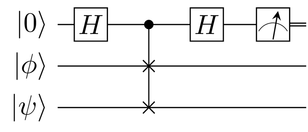
The inner product can be estimated with the SWAP-test.

SWAP test circuit, taken from Wikipedia.

The inner product estimate is calculated from

\[ P(\text{control qubit} = 0) = \frac{1}{2} + \frac{1}{2}\lvert\langle \psi | \phi \rangle\rvert^2 \]

Implementation

In this implementation, each feature vector is normalized, and since each vector has dimension two, a single qubit suffices to encode the data.

from pennylane import numpy as np
import pennylane as qml


def distance(A, B):
    """Function that returns the distance between two vectors.

    Args:
        - A (list[int]): person's information: [age, minutes spent watching TV].
        - B (list[int]): person's information: [age, minutes spent watching TV].

    Returns:
        - (float): distance between the two feature vectors.
    """

    def prep_state():
        """Function that encodes the two 2D feature vectors into the amplitudes of one qubit each."""
        
        tan_thetaA = A[0]/A[1]
        thetaA = np.arctan(tan_thetaA)
        tan_thetaB = B[0]/B[1]
        thetaB = np.arctan(tan_thetaB)
        
        qml.RY(2.*thetaA, wires=0)
        qml.RY(2.*thetaB, wires=1)
    
    
    dev = qml.device("default.qubit", wires=3)
    @qml.qnode(dev)
    def circuit():
        """Quantum circuit that encodes two 2D-feature vectors and performs a SWAP test.
        
        Returns:
            - ([float, float]): probabilities of states measured on the control qubit.
        """
        prep_state()
        
        qml.Hadamard(wires=2)
        qml.CSWAP(wires=range(2,-1,-1))
        qml.Hadamard(wires=2)
        
        return qml.probs(2)

    # print(qml.draw(circuit)())
    
    tmp = circuit()[0] # .5 + .5<A,B>^2
    A_times_B = np.sqrt(2.*tmp-1.)
    
    return np.sqrt(2*(1.-A_times_B))

The provided tests check out.

Lessons learned

I will seize this opportunity to reflect upon my solution strategies. The problem statement was a little less concrete than the ones of previous exercises. In the starter code two hints were pointing at the SWAP Test and the PennyLane amplitude encoding functionality. After an initial implementation failed, I did some more research and found a SWAP-test implementation on a PennyLane forum. This was more confusing then helpful, I believe the core confusion being how the normalization is done in this encoding strategy.

Anyways, the clean bottom up solution, along with some debugging print-outs eventually worked out.

QHack 2023: 4 week prep challenge, day 13, A Quantum Algorithm

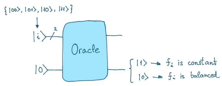
After having a rest day yesterday, today, I’m continuing with the most advanced exercise on the algorithms track. The task is an extension to the Deutsch-Jozsa algorithm. You are given four individual functions, of which either all four are equally balanced/constant or two are balanced and two are constant. The algorithm has to decide which case is materialized, using no more than 8 qubits.

Depiction of the oracle, taken from here.

Now, I think it is easiest to evaluate the functions one by one, and sum up the result bits using the QFT-adder logic from a previous exercise and distinguish the cases depending on the resulting count.

Optimizing for gate count

If you want to minimize the gate count, you can perform each function once, writing the results of each function to individual qubits. Eventually, you can make controlled increments on a two qubit register (mod 4), where each wire serves as a control. You need 8 qubits in total

  • two input qubits
  • four qubits to store the function results
  • two qubits for the counter

You have three possible cases:

  • Four balanced functions, no increments are performed, the counter register reads |00>
  • Four constant functions, four increments are performed, the counter register overflows and eventually reads |00>
  • Two balanced functions and two constant functions, the counter register reads |10>

Optimizing for qubit number

If you want to minimize the number of qubits needed, I came up with a similar solution that uses only four qubits:

  • two input qubits
  • one control qubit
  • one qubit for the counter

With the known two possible result cases, you can opt to make half increments, instead of full increments, this reduces the counter register size by one qubit.

After performing the controlled counting, you can undo the oracle operation by applying the inverse and therefore freeing up the control qubit for further use.

Here is my code, doing just that …

def deutsch_jozsa(fs):
    """Function that determines whether four given functions are all of the same type or not.

    Args:
        - fs (list(function)): A list of 4 quantum functions. Each of them will accept a 'wires' parameter.
        The first two wires refer to the input and the third to the output of the function.

    Returns:
        - (str) : "4 same" or "2 and 2"
    """

    dev = qml.device("default.qubit", wires=4, shots=1)
    inp_wires = range(2)
    
    def controlled_half_increment(crtl_wire, wire):
        """Quantum function capable of performing a half increment on a single qubit (i.e. mod 1)

        Args:
            - ctrl_wire (int): wire to control the operation
            - wire (int): wire on which the function will be executed on.
        """

        wires = [wire, ]
        qml.QFT(wires=wires)

        qml.CRZ(np.pi/2, wires=[crtl_wire, wires[0]])

        qml.adjoint(qml.QFT)(wires=wires)
    
    @qml.qnode(dev)
    def circuit():
        """Implements the modified Deutsch Jozsa algorithm."""
        
        qml.broadcast(qml.Hadamard, wires=inp_wires, pattern="single")

        for f in fs:
            f(range(3))
            controlled_half_increment(2,3)
            qml.adjoint(f)(range(3))
        
        qml.broadcast(qml.Hadamard, wires=inp_wires, pattern="single") # this is 

        return qml.sample(wires=[3,]) # 1 .. 2 and 2, 0 .. 4 the same

    sample = circuit()
    
    four_same = "4 same"
    two_and_two = "2 and 2"
    
    return four_same if sample == 0 else two_and_two

Testing the algorithm

The starter code includes a scheme for generating the functions. First, I tested the code, by passing the provided test data to the algorithm – but to me it looked like the results were published wrong. I continued by passing the same function four times – checks out, and then passing combinations of two functions – and ended up observing both cases: equal situations and two and two situations. I took it for a successful test.

QHack 2023: 4 week prep challenge, day 12, Quantum Counting

I continued on the quantum algorithms track, with the quantum counting exercise. The number of solutions to a search problem should be estimated using Grover search and Quantum Phase Estimation.

I’ve found a very concise and clear video on Grover’s algorithm and the accompanying basic example code.

The coding itself boiled down to some basic numpy matrix wrangling, and implementing the proposed algorithm. A more detailed description of the solution scheme can be found here.

Since I had a little more time, I also read up on QFT arithmetics. I wasn’t aware of the tutorial yesterday, it would have been very helpful though!

QHack 2023: 4 week prep challenge, day 11, A Quantum Adder (QFT)

Today, I’m continuing with the next exercise from the algorithms track. The task is to build a number adder using the Fourier space.

Firstly, a Fourier transform is applied on the initial state, i.e. a state |0> or |1> in the computational basis is flipped into the X-Y-plane. The qubits are then rotated around the Z-axis, with an angle according to the number to add. Eventually, the state is transformed back from the Fourier space.

The transformation rule for the QFT reads

\[ QFT|x\rangle = \frac{1}{\sqrt{M}} \sum^{M-1}_{k=0} \exp(\frac{2 \pi i}{M} x k) |k\rangle \]

If you now want to add to a state in the Fourier space, you have to rotate the qubits accordingly. It is important to notice, that a rotation only effects the |1> portion, but not the |0> portion of a qubit’s state.

Having that in mind, it was relatively straight forward to come up with the solution…

def qfunc_adder(m, wires):
    """Quantum function capable of adding m units to a basic state given as input.

    Args:
        - m (int): units to add.
        - wires (list(int)): list of wires in which the function will be executed on.
    """

    qml.QFT(wires=wires)

    for w, _ in enumerate(wires):
        angle = m*np.pi/(2**w)
        qml.RZ(angle, wires=w)

    qml.QFT(wires=wires).inv()

… the tests check out, success!

QHack 2023: 4 week prep challenge, day 10, A topology survey

I continued on the Algorithm track with the adapting topologies exercise. It is an easy, but very enjoyable task, I just really like working with graphs.

Topology

Quanta need to be next to each other, when performing multi-qubit operations like CNOT, SWAP, etc. on them. If you want to perform a multi-qubit operation on non-adjacent qubits, you’ve got to SWAP them around, until they are next to each other. Therefore, a higher connectivity is beneficial to save up coherence for the main calculations.

However, operations on qubits may cause cross-talk on neighboring qubits, and therefore reducing coherence.

Now the topology of a QPU has to weigh-in both effects, and there are topologies that optimize for reduced cross-talk (e.g. ion traps), maximal connectivity, or seek to balance the two (e.g. IBM’s heavy hexagonal lattice).

Exercise

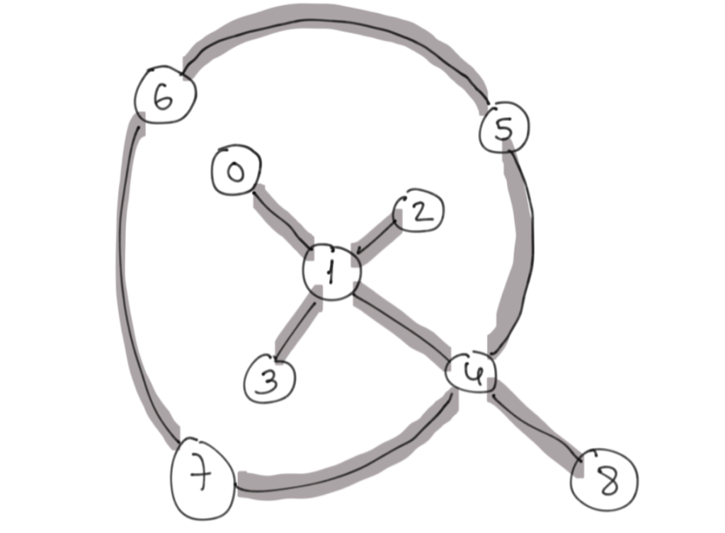
Now in this exercise, a toy topology is provided, and the challenge is to calculate the number of SWAPs required to perform a CNOT gate. For this, I used the python library networkx.

Toy topology, taken from here.
import networkx as nx

def get_topology_graph():
    """Create an adjacency graph, of the topology dict.
    
    Args:
    
    Returns: 
        - (nx.Graph): adjacency graph
    """
    
    G = nx.Graph()
    
    for i, nodes in graph.items():
        elist = [(i, j) for j in nodes]
        G.add_edges_from(elist)
    
    return G

The SWAP count, is then easily calculated from the length of the shortest path (don’t forget to rewind the operations, to clean up after the CNOT).

def n_swaps(cnot):
    """Count the minimum number of swaps needed to create the equivalent CNOT.

    Args:
        - cnot (qml.Operation): A CNOT gate that needs to be implemented on the hardware
        You can find out the wires on which an operator works by asking for the 'wires' attribute: 'cnot.wires'

    Returns:
        - (int): minimum number of swaps
    """
    
    G = get_topology_graph()
    wires = cnot.wires
    path = nx.shortest_path(G, wires[0], wires[1])
    
    return 2*(len(path)-2)

The results check out, success!

Plotting a sample circuit

To round the story up, I wrote a small routine to build out a circuit, that actually swaps the qubits around ..

dev = qml.device("default.qubit", wires=len(graph))

@qml.qnode(dev)
def n_swaps_perf(wire1, wire2):
    G = get_topology_graph()
    
    path = nx.shortest_path(G, wire1, wire2)
    path.pop(-1) # remove last item, to have easier indexing in loops
    
    for i in range(1, len(path)):
        qml.SWAP(wires=[path[i], path[i-1]])
        
    qml.CNOT(wires=[path[-1], wire2])
    
    rev_path = list(reversed(path))
    
    for i in range(1, len(rev_path)):
        qml.SWAP(wires=[rev_path[i], rev_path[i-1]])
        
    return qml.expval(qml.PauliZ(wires=wire2))

.. and plots the resulting circuit.

drawer = qml.draw(n_swaps_perf)
print(drawer(8,2))
1: ───────╭SWAP─╭●─╭SWAP───────┤     
2: ───────│────╰X─│───────────┤  <Z>
4: ─╭SWAP─-╰SWAP────╰SWAP─╭SWAP─-┤     
8: ─╰SWAP────────────────╰SWAP─┤     

Looks good.