Today is a very tired day, I just solved the easiest puzzle from the Algorithms track to keep the rhythm. Deutsch Josza algorithm.
Meanwhile, I registered for the iQuHack event this weekend. It is organized by people associated with the MIT and Microsoft is a sponsor of the remote-track. I plan to take a look through resources from the previous years, and probably a few Q# resources to have a rough idea what is awaiting me, and possibly have a more enjoyable experience.
Tag: Quantum Computing
QHack 2023: 4 week prep challenge, day 8, Pennylane 101
I’m struggling with the next exercise (Who likes the beatles, k-NN) on the ML track, I will have to read up on embeddings and the swap test. My web search lead me to this Pennylane forum entry, but the proposed solution looks not quite right to me. Well, after some coding and some tests, I decided I was too tired to do the harder reading and opted to solidify some concepts and solve a few easier exercises instead. On the Pennylane 101-track, I solved the exercises 1, 2, 3, and 4. Following, are a few thoughts I had along the way…
Ad Exercise 1, gate order
The exercise highlighted the non-commuting nature of operators.
Ad Exercise 2, devices
Pennylane offers multiple (simulation) devices to choose from, a brief listing
- default device
- devices to use in combination with ML frameworks (JAX, PyTorch, TensorFlow)
- device for mixed state calculations
- device for Quitrits. Quitrits enable calculations in a three-valued logic, there may be some physical advantages to such systems (stability, …), but I picture quite some mental gymnastics to deal with them.
Ad Exercise 3, superdense coding
With super dense coding, it is possible to send 2-bits of information, while transmitting only one qubit after defining the message (One entangled qubit without information is sent before defining the message).
To solve the exercise, I used a RY gate to emulate a noisy Hadamard gate.
Interesting to me, was the qml.broadcast command, that offers a number of handy wiring patterns, and will spare me a few loops in the future.
Ad Exercise 4, finite difference method
For VQE optimizations, it is essential to have the gradients of a given circuit. Differentiability is generally a very important aspect of the Pennylane library. It is worthwhile to recap the different differentiation methods:
- backprop
- adjoint
- parameter-shift
- finite-diff
These options also enter my reading list.
QHack 2023: 4 week prep challenge, day 6, H-H first excited state
Almost a week passed, it’s time for more tricky tasks! The last and most advanced exercise in the Quantum Chemistry track of the 2022 QHack.
Disclaimer: At the time being, the proposed solution does not produce the correct results.
The task is to obtain the energy of the first excited state of an H-H molecule at a given nuclei distance. This is achieved by firstly calculating the ground state energy, and later modifying the systems Hamiltonian to penalize the actual ground state. Repeating the ground-state calculation with the modified Hamiltonian, you can obtain the first excited state.
The calculation of the ground-state via a VQE routine, is done following the concise Pennylane VQE tutorial, with only minuscule modifications.
import sys
import pennylane as qml
from pennylane import numpy as np
from pennylane import hf


def ground_state_VQE(H):
    """Perform VQE to find the ground state of the H2 Hamiltonian.

    Args:
        - H (qml.Hamiltonian): The Hydrogen (H2) Hamiltonian

    Returns:
        - (float): The ground state energy
        - (np.ndarray): The ground state calculated through your optimization routine
    """

    qubits = 4

    dev = qml.device("default.qubit", wires=qubits)

    electrons = 2
    hf = qml.qchem.hf_state(electrons, qubits)

    def circuit(param, wires):
        qml.BasisState(hf, wires=wires)
        qml.DoubleExcitation(param, wires=range(qubits))

    @qml.qnode(dev)
    def cost_fn(param):
        circuit(param, wires=range(qubits))
        return qml.expval(H)

    @qml.qnode(dev)
    def ground_state(param, wires):
        circuit(param, wires)
        return qml.state()

    opt = qml.GradientDescentOptimizer(stepsize=0.1)
    theta = np.array(0.0, requires_grad=True)

    # store the values of the cost function
    energy = [cost_fn(theta)]

    # store the values of the circuit parameter
    angle = [theta]

    max_iterations = 100
    conv_tol = 1e-06

    for n in range(max_iterations):
        theta, prev_energy = opt.step_and_cost(cost_fn, theta)

        energy.append(cost_fn(theta))
        angle.append(theta)

        conv = np.abs(energy[-1] - prev_energy)

        if n % 2 == 0:
            print(f"Step = {n},  Energy = {energy[-1]:.8f} Ha, theta = {theta:.3f}")

        if conv <= conv_tol:
            break

    E0 = energy[-1]
    gstate = ground_state(theta, wires=range(qubits))

    return E0, gstate

symbols = ["H", "H"]
coord = 0.6614
geometry = np.array([[0.0, 0.0, -coord], [0.0, 0.0, coord]], requires_grad=False)
mol = hf.Molecule(symbols, geometry)

H = hf.generate_hamiltonian(mol)()
E0, ground_state = ground_state_VQE(H)
The next step is to calculate a modified Hamiltonian.
def create_H1(ground_state, beta, H):
    """Create the H1 matrix, then use `qml.Hermitian(matrix)` to return an observable-form of H1.

    Args:
        - ground_state (np.ndarray): from the ground state VQE calculation
        - beta (float): the prefactor for the ground state projector term
        - H (qml.Hamiltonian): the result of hf.generate_hamiltonian(mol)()

    Returns:
        - (qml.Observable): The result of qml.Hermitian(H1_matrix)
    """

    H1 = qml.matrix(H) + beta * np.outer(ground_state, ground_state)
    qubits = int(np.log2(len(ground_state)))
    return qml.Hermitian(H1, wires=range(qubits))


def excited_state_VQE(H1):
    """Perform VQE using the "excited state" Hamiltonian.

    Args:
        - H1 (qml.Observable): result of create_H1

    Returns:
        - (float): The excited state energy
    """

    E1, estate = ground_state_VQE(H1)
    return E1

beta = 15.0
H1 = create_H1(ground_state, beta, H)
E1 = excited_state_VQE(H1)

print(E1)
While the ground state energy is correctly calculated, some error remains in the calculation of the excited state energy (larger than zero). … I will leave it to rest for the next few days, and maybe revisit it later.
QHack 2023: 4 week prep challenge, day 5, Triple excitation Givens rotation
Continuing on the Quantum Chemistry track, the next exercise. According to the designers, it is more difficult than the last ones, but it suited me very well. With the knowledge of the previous days, I could solve the task by merely looking at it.
The task is to prepare the state
\[ |\psi(\alpha, \beta, \gamma)\rangle =
\cos{\frac{\alpha}{2}} \cos{\frac{\beta}{2}} \left[ \cos{\frac{\gamma}{2}} |111000\rangle – \sin{\frac{\gamma}{2}}|000111\rangle \right] –
\cos{\frac{\alpha}{2}} \sin{\frac{\beta}{2}}|001011\rangle –
\sin{\frac{\alpha}{2}} |011001\rangle
\]
using a single excitation, a double excitation and a triple excitation, the latter one should be constructed from a matrix.
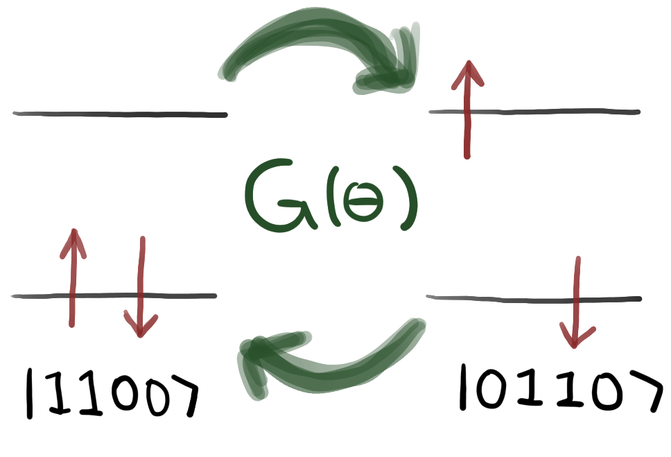
Constructing a triple excitation Givens rotation
This is a really straight forward task. The transformation rules are analogous to the single and double excitations
\[
G^{(3)}(\gamma)|000111\rangle = \cos{\frac{\gamma}{2}} | 000111\rangle + \sin{\frac{\gamma}{2}} |111000\rangle \\
G^{(3)}(\gamma)|111000\rangle = \cos{\frac{\gamma}{2}} | 111000\rangle – \sin{\frac{\gamma}{2}} |000111\rangle
\]
and the realization, that the decimal representations of the states provide you with the target indices in the transformation matrix
\[
|000111\rangle = |7\rangle, \\
|111000\rangle = |56\rangle
\]
yields the implementation
def triple_excitation_matrix(gamma):
    """The matrix representation of a triple-excitation Givens rotation.
https://github.com/XanaduAI/QHack2022/tree/master/Coding_Challenges/qchem_400_TripleGivens_template
    Args:
        - gamma (float): The angle of rotation

    Returns:
        - (np.ndarray): The matrix representation of a triple-excitation
    """

    dim = 2**6
    res = np.identity(dim)

    # |000111> = |7>
    # G3(theta)|7> = cos(theta/2)|7> + sin(theta/2)|56>
    row7 = np.zeros(dim)
    row7[7] = np.cos(gamma/2)
    row7[56] = -np.sin(gamma/2)

    # |111000> = |56>
    # G3(theta)|56> = cos(theta/2)|56> - sin(theta/2)|7>
    row56 = np.zeros(dim)
    row56[7] = np.sin(gamma/2)
    row56[56] = np.cos(gamma/2)

    res[7] = row7
    res[56] = row56

    return res
Preparing the target state
This was solved by looking at the states and the pre-factors. The basis-states with a single pre-factor underwent only a single Givens rotation…
@qml.qnode(dev)
def circuit(angles):
    """Prepares the quantum state in the problem statement and returns qml.probs

    Args:
        - angles (list(float)): The relevant angles in the problem statement in this order:
        [alpha, beta, gamma]

    Returns:
        - (np.tensor): The probability of each computational basis state
    """

    # QHACK #
    qml.BasisState(np.array([1, 1, 1, 0, 0, 0]), wires=[0, 1, 2, 3, 4, 5])
    qml.SingleExcitation(angles[0], wires=[0, 5])
    qml.DoubleExcitation(angles[1], wires=[0,1,4,5])
    qml.QubitUnitary(triple_excitation_matrix(angles[2]), wires=[0,1,2,3,4,5])
    # QHACK #

    return qml.probs(wires=range(NUM_WIRES))
The provided test datasets yield the correct results, success!
QHack 2023: 4 week prep challenge, day 4, Givens rotations
Today, I’m heading again for a prepared exercise, the next exercise in the QHack 2022 Quantum Chemistry track. It requires slightly more preparation, than the previous two, but again very doable.
The challenge, invites to get more acquainted with Givens rotations, i.e. operations that allow to transform states, while preserving the hamming weight (the number of ones and zeros). They are the basic building blocks of quantum chemistry and “can be used to construct any kind of particle-conserving circuit”.
The goal is to find the correct rotation angles to transform a start state to a target state, with a quantum circuit with three Givens rotations,
\[|\Psi \rangle = CG^{(1)}(\theta_3; 0,1,3) G^{(2)}(\theta_2; 2,3,4,5) G^{(2)}(\theta_1; 0,1,2,3) |110000\rangle = \\ a |110000\rangle + b |001100 \rangle + c |000011 \rangle + d |100100\rangle \]
Getting to know Givens rotations
Givens rotations, describe transitions of electrons from a starting state to an excited state. In Pennylane, these rotations can be used via the classes qml.SingleExcitation and qml.DoubleExcitation. The linked tutorial is very recommendable.
Solving the exercise
To solve this exercise, I used the rotations’ transformation rules to reach an expression that associated trigonometric functions with the target factors. Further, I used the fact, that states are normalized at any time during the calculation. Key for me to solve it, was to apply only the first two rotations and used the normalization property of the state, from this I obtained the first angle. Then I went on to apply the remaining rotation and easily expressed the missing two angles.
import numpy as np


def givens_rotations(a, b, c, d):
    """Calculates the angles needed for a Givens rotation to out put the state with amplitudes a,b,c and d

    Args:
        - a,b,c,d (float): real numbers which represent the amplitude of the relevant basis states (see problem statement). Assume they are normalized.

    Returns:
        - (list(float)): a list of real numbers ranging in the intervals provided in the challenge statement, which represent the angles in the Givens rotations,
        in order, that must be applied.
    """

    theta1 = 2.*np.arccos(np.sqrt(1-b**2-c**2))
    theta2 = 2.*np.arcsin(c/np.sin(theta1/2.))
    theta3 = 2.*np.arccos(a/np.cos(theta1/2.))

    return [theta1, theta2, theta3]
Test
Defining the circuit…
import pennylane as qml

dev = qml.device('default.qubit', wires=6)

@qml.qnode(dev)
def circuit(x, y, z):
    qml.BasisState(np.array([1, 1, 0, 0, 0, 0]), wires=[i for i in range(6)])
    qml.DoubleExcitation(x, wires=[0, 1, 2, 3])
    qml.DoubleExcitation(y, wires=[2, 3, 4, 5])
    # single excitation controlled on qubit 0
    qml.ctrl(qml.SingleExcitation, control=0)(z, wires=[1, 3])
    return qml.state()
and executing the circuit …
[x, y, z] = givens_rotations(0.8062,-0.5,-0.1,-0.3)
circuit(x,y,z)
yields the correct amplitudes, success!
Transformation rules
Double excitation
\[ G^{(2)} (\theta; 1,2,3,4) |0011\rangle = \cos{\frac{\theta}{2}} |0011\rangle + \sin{\frac{\theta}{2}} |1100\rangle \\
G^{(2)} (\theta; 1,2,3,4) |1100\rangle = \cos{\frac{\theta}{2}} |1100\rangle – \sin{\frac{\theta}{2}} |0011\rangle \\
\]
Controlled single excitation
\[
CG(\theta; 0,1,2)|101\rangle = \cos{\frac{\theta}{2}}|101\rangle + \sin{\frac{\theta}{2}}|110\rangle \\
CG(\theta; 0,1,2)|110\rangle = \cos{\frac{\theta}{2}}|110\rangle – \sin{\frac{\theta}{2}}|101\rangle
\]
Through the year with Quantum Computing
The most important quantum computing learning events for beginners and intermediates.
The most important quantum computing learning events for beginners and intermediates.
I missed some learning opportunities in my first few months into quantum computing, I wrote this post, to help you do better than me!
As a beginner myself, I am continuously searching for learning opportunities and for opportunities to connect with like-minded people. Outside academia, Quantum Computing is a relatively young technology. Tools and resources are continuously created to help a broader audience to get into the field.
There is a range of easily accessible offerings from various Quantum Computing providers and organizations. I personally found many tutorials and their respective problem statements very abstract, and difficult to relate to. So I looked out for more interactive learning formats.
Online hackathons (e.g. by IBM Quantum or by Pennylane) are ideal for hands-on learning of algorithms, frameworks and key-concepts. They are often very well curated, (apart from some bare basics) provide all the information needed to complete the challenges, but require you to study the provided materials closely. Furthermore, they might come with a message board, to connect with people in your area.
That being said, my personal experience with the hackathons was, that they are oftentimes announced at short notice, and it’s easy to miss out on them. However, you can join on the spot, no preparation strictly required (some basics of the target framework are highly recommended though).
More advanced people may look out to join a dedicated mentorship program, like the one by OQSF, or for offerings that require applicants to demonstrate a lot more work for the community, like the Qiskit Advocate program. These advanced programs need much more preparation and planning.
I attached a small overview of offerings I found, and when they took place in the past. Application deadlines to restricted offerings precede the event some time – so be careful with these.
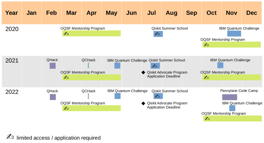
I enjoyed doing hackathons a lot, and with this overview you too should be able to anticipate them. If you still miss one – don’t worry, the resources are usually published with some delay on github, so you can enjoy the contents out of competition. There’s always a next event around the corner, so keep at it!